Examples

This section gives some examples for how the package can be used. We consider the same type of initial condition, migration, and prloiferation mechanisms, but break the example into four parts:

Fixed boundaries, no proliferation;
Fixed boundaries, proliferation;
Free boundaries, no proliferation;
Free boundaries, proliferation.

The initial condition we use is a step function density on $0 \leq x \leq 30$, with cells in $[0, 15]$ of low density and cells in $[15, 30]$ of great density:

initial_condition = [LinRange(0, 15, 16); LinRange(15, 30, 32)] |> unique!
fig = Figure(fontsize=33)
ax = Axis(fig[1, 1], xlabel=L"x",width=600,height=200)
scatter!(ax, initial_condition, zero(initial_condition),color=:black,markersize=13)
hideydecorations!(ax)
resize_to_layout!(fig)
fig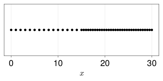

When considering cell migration, the force law we use is the linear law $F(\delta) = k(s - \delta)$, where $k = 10$ is the spring constant in each example, and $s = 0.2$ is the resting spring length except in the last example where $s=1$. When including proliferation, we use the logistic law $G(\delta) = \beta[1 - 1/(K\delta)]$, where $\beta = 0.15$ is the intrinsic proliferation rate and $K=15$ is the cell carrying capacity density. This choice of proliferation law slows down the growth of a cell population when there are many cells packed together, ensuring that a steady state can be reached (when there is no moving boundary). (To see that this is a logistic law, note that in the continuum limit the corresponding reaction term is $qG(1/q) = \beta q[1 - q/K]$, which is the same term in the Fisher equation.)

Example I: Fixed boundaries, no proliferation

We start with a problem that fixes both boundaries and only includes cell migration. The first step we take is to define the problem itself:

using EpithelialDynamics1D 
force_law = (δ, p) -> p.k * (p.s - δ)
force_law_parameters = (k=10.0, s=0.2)
final_time = 100.0
damping_constant = 1.0
initial_condition = [LinRange(0, 15, 16); LinRange(15, 30,32)] |> unique!
prob = CellProblem(;
    force_law,
    force_law_parameters,
    final_time,
    damping_constant,
    initial_condition)

This problem can be solved like any other problem from DifferentialEquations.jl. I find that Tsit5() is typically the fastest:

using OrdinaryDiffEq
sol = solve(prob, Tsit5(), saveat=10.0)

Let's compare this solution to its continuum limit. From Baker et al. (2019), the continuum limit is given by

\[\begin{align*} \begin{array}{rcll} \dfrac{\partial q}{\partial t} & = & \dfrac{\partial}{\partial x}\left(D(q)\dfrac{\partial q}{\partial x}\right) & 0 < x < L,\,t>0,\\[9pt] \dfrac{\partial q}{\partial x} & = & 0 & x = 0,\,t>0,\\[9pt] \dfrac{\partial q}{\partial x} & = & 0 & x = L,\,t>0,\\[9pt] q(x, 0) & = & q_0(x) & 0 \leq x \leq L. \end{array} \end{align*}\]

These PDEs are solved using FiniteVolumeMethod1D.jl. This dependent variable $q$ is the cell density. There are two possible ways to define densities:

cell_densities: The cell_densities function defines the density of a cell $(x_i, x_{i+1})$ as the reciprocal length $q_i = 1/(x_{i+1} - x_i)$.
node_densities: The node_densities function, the one that actually gets used in the continuum limit, assigns densities to nodes $x_i$ rather than cells $(x_i, x_{i+1})$. The density at a node $x_i$ is defined by $q_i = 2/(x_{i+1} - x_{i-1})$ if $1 < i < n$, where $n$ is the number of cells at the given time, or $q_1 = 1/(x_2 - x_1)$ and $q_n = 1/(x_n - x_{n-1})$ at the endpoints.

The latter definition is used in the continuum limit - the initial condition $q_0(x)$ is a piecewise linear interpolant through the cell densities at the initial time from the cell problem's initial condition. The diffusion function $D(q)$ is given by

\[D(q) = -\dfrac{1}{\eta q^2}F'\left(\dfrac{1}{q}\right),\]

which for our force law is $D(q) = \alpha/q^2$, $\alpha = k/\eta$.

The function continuum_limit constructs the FVMProblem defining this continuum limit:

fvm_prob = continuum_limit(prob, 1000)

The second argument 1000 defines the number of mesh points to use for the continuum limit, using the piecewise linear interpolant $q_0(x)$ to compute the densities at each mesh point. Now let's solve it:

using LinearSolve
fvm_sol = solve(fvm_prob, TRBDF2(linsolve=KLUFactorization()), saveat=10.0)

If the simulation is correct, noting that our value of $k$ is sufficiently high so that the continuum limit should actually work, then fvm_sol should be a good match to the densities from sol. To verify this, let us make a plot:

node_densities_sol = node_densities.(sol.u)
using CairoMakie
let x = fvm_prob.geometry.mesh_points
    fig = Figure(fontsize=36)
    colors = (:red, :blue, :darkgreen, :black, :orange, :magenta,:cyan, :yellow, :brown, :gray, :lightblue)
    ax = Axis(fig[1, 1], xlabel=L"x", ylabel=L"q(x, t)",
        title=L"(a): $q(x, t)$", titlealign=:left,
        width=600, height=300)
    [lines!(ax, sol.u[i], node_densities_sol[i], color=colors[i],linewidth=2) for i in eachindex(sol)]
    [lines!(ax, x, fvm_sol.u[i], color=colors[i], linewidth=4,linestyle=:dashdot) for i in eachindex(sol)]
    resize_to_layout!(fig)
    fig
end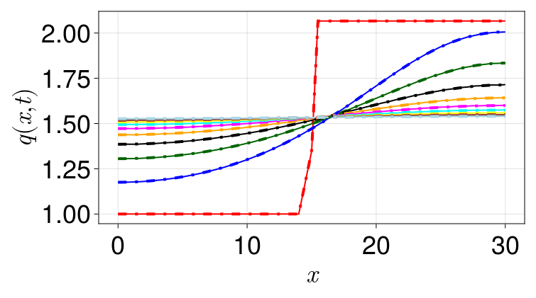

We see that the continuum limit lines up perfectly with the discrete results, and the solution approaches the steady state that is the average of the two densities from the initial condition. We provide a SteadyCellProblem for computing this steady state without running any simulation:

using SteadyStateDiffEq
sprob = SteadyCellProblem(prob)
ssol = solve(sprob, DynamicSS(TRBDF2()))
q = cell_densities(ssol.u)

julia> q = cell_densities(ssol.u)
46-element Vector{Float64}:
 1.5333521372657852
 1.533352049592097
 1.5333518746535277
 1.5333516132657792
 1.5333512666476505
 ⋮
 1.533315400438977
 1.5333150538372589
 1.5333147924620867
 1.5333146175320538
 1.5333145298626596

Example II: Moving boundary, no proliferation

Now let's allow the rightmost boundary to be free. This is done by setting fix_right = false in the CellProblem constructor.

using EpithelialDynamics1D, OrdinaryDiffEq

force_law = (δ, p) -> p.k * (p.s - δ)
force_law_parameters = (k=10.0, s=0.2)
final_time = 500.0
damping_constant = 1.0
initial_condition = [LinRange(0, 15, 16); LinRange(15, 30, 32)] |>unique!
prob = CellProblem(;
    force_law,
    force_law_parameters,
    final_time,
    damping_constant,
    initial_condition,
    fix_right=false)

sol = solve(prob, Tsit5(), saveat=50.0)

The continuum limit that we can compare to in this case is this given by, letting $L(t)$ denote the position of the rightmost node (the leading edge) at the time $t$.

\[\begin{align*} \begin{array}{rcll} \dfrac{\partial q}{\partial t} & = & \dfrac{\partial}{\partial x}\left(D(q)\dfrac{\partial q}{\partial x}\right) & 0 < x < L(t),\,t>0,\\[9pt] \dfrac{\partial q}{\partial x} & = & 0 & x = 0, \\[9pt] \dfrac{1}{\eta}F\left(\dfrac{1}{q}\right) + \dfrac{D(q)}{2q}\dfrac{\partial q}{\partial x} & = & 0 & x=L(t),\.t>0,\\[9pt] \dfrac{\mathrm dL}{\mathrm dt} & = & -\dfrac{1}{q}D(q)\dfrac{\partial q}{\partial x} & x = L(t),\,t>0, \\[9pt] q(x, 0) & = & q_0(x), & 0 \leq x \leq L(0), \\[9pt] L(0) & = & L_0. \end{array} \end{align*}\]

These PDEs are solved using MovingBoundaryProblems1D.jl. The initial endpoint $L_0$ is given by the position of the rightmost node at $t=0$, in this case $L_0 = 30$. Once again, we construct the corresponding problem, in this case an MBProblem, using continuum_limit:

using LinearSolve

mb_prob = continuum_limit(prob, 1000)
mb_sol = solve(mb_prob, TRBDF2(linsolve=KLUFactorization()), saveat=50.0)

The following code then plots and compares the two solutions.

node_densities_sol = node_densities.(sol.u)
using CairoMakie
let x = mb_prob.geometry.mesh_points
    fig = Figure(fontsize=36)
    colors = (:red, :blue, :darkgreen, :black, :orange, :magenta,:cyan, :yellow, :brown, :gray, :lightblue)
    ax = Axis(fig[1, 1], xlabel=L"x", ylabel=L"q(x, t)",
        title=L"(a): $q(x, t)$", titlealign=:left,
        width=600, height=300)
    [lines!(ax, sol.u[i], node_densities_sol[i], color=colors[i],linewidth=2) for i in eachindex(sol)]
    @views [lines!(ax, x .* mb_sol.u[i][end], mb_sol.u[i][begin(end-1)], color=colors[i], linewidth=4, linestyle=:dashdot)for i in eachindex(sol)]
    resize_to_layout!(fig)
    fig
end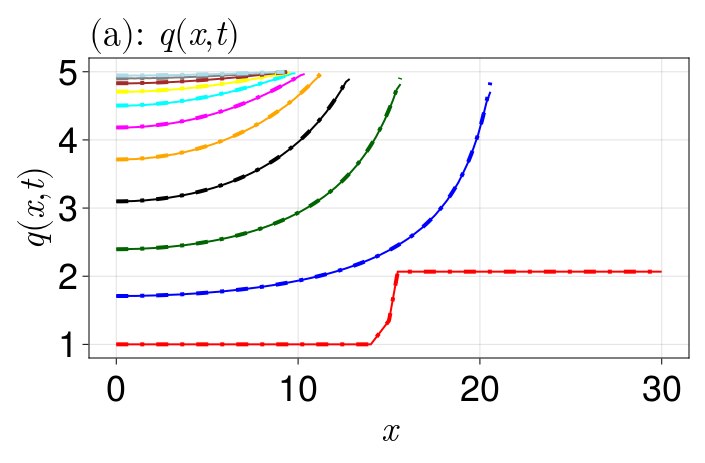

We see that the solutions match. The cells appear to be retreating from $L(0) = 30$, contracting inwards until a steady state is eventually reached. In this steady state, the cells seem to pack into the interval $[0, 10]$. This makes sense - we start with 46 cells:

julia> length(initial_condition) - 1
46

With a resting spring length of $s = 0.2$, we can fit 46 cells into the interval $[0, 46 \cdot 0.2] = [0, 9.2]$. We can verify the properties of this steady state by either looking at the last time from the simulation, or by computing the steady state directly:

julia> diffs = diff(sol.u[end])
46-element Vector{Float64}:
 0.20233969090471757
 0.20203667605421724
 0.20263100257524164
 0.20172744674985177
 0.20290519447397481
 ⋮
 0.19964286225916084
 0.20089946315869867
 0.1997809643420574
 0.20045281417783656
 0.19992619110920273

Indeed, the length of each cell is approximately $s = 0.2$, and the endpoint at the last time is:

julia> sol.u[end][end]
9.267001076147542

which is approaching $9.2$. If we look at the steady state:

using SteadyStateDiffEq 
sprob = SteadyCellProblem(prob)

julia> ssol = solve(sprob, DynamicSS(TRBDF2()))
u: 47-element Vector{Float64}:
 -3.8321946143843015e-20
  0.20000125473810257
  0.4000025080445262
  0.6000037584892256
  0.8000050046454205
  ⋮
  8.400036722439138
  8.600036891490856
  8.800037018448712
  9.000037103167848
  9.200037145551596

We see that the cells all have lengths approximately equal to $s$, and $\lim_{t \to \infty} L(t) = 9.2$ as predicted.

Example III: Fixed boundary, with proliferation

Now let us go back to the fixed boundary problem, but now include proliferation. Remember that the proliferation law we use is the logistic law $G(\delta) = \beta[1 - 1/(K\delta)]$.

The procedure for solving problems with proliferation is different than without. Since the proliferation mechanism is stochastic, we need to simulate the system many times to capture the average behaviour. We use the ensemble solution features from DifferentialEquations.jl to do this, using the trajectories keyword to specify how many simulations of the systems we want.

using EpithelialDynamics1D, OrdinaryDiffEq 

force_law = (δ, p) -> p.k * (p.s - δ)
force_law_parameters = (k=10.0, s=0.2)
proliferation_law = (δ, p) -> p.β * (one(δ) - inv(p.K * δ))
proliferation_law_parameters = (β=0.15, K=15.0)
proliferation_period = 1e-2
final_time = 50.0
damping_constant = 1.0
initial_condition = [LinRange(0, 15, 16); LinRange(15, 30, 32)] |>unique!
prob = CellProblem(;
    force_law,
    force_law_parameters,
    proliferation_law,
    proliferation_law_parameters,
    proliferation_period,
    final_time,
    damping_constant,
    initial_condition)
ens_prob = EnsembleProblem(prob)
sol = solve(ens_prob, Tsit5(); trajectories=50, saveat=0.01)

The continuum limit for this problem is similar to the problem without proliferation, except the PDE has a reaction term:

\[\dfrac{\partial q}{\partial t} = \dfrac{\partial}{\partial x}\left(D(q)\dfrac{\partial q}{\partial x}\right) + qG\left(\dfrac{1}{q}\right);\]

the other boundary and initial conditions are the same as in the first example. As in the first example, PDEs of this form are solved using FiniteVolumeMethod1D.jl.

using LinearSolve 

fvm_prob = continuum_limit(prob, 1000; proliferation=true)
fvm_sol = solve(fvm_prob, TRBDF2(linsolve=KLUFactorization()), saveat=0.01)

Note that the proliferation=true keyword argument is needed in continuum_limit, else the continuum limit without proliferation is returned.

We provide several functions for computing statistics from the EnsembleSolution, sol. The function node_densities returns a NamedTuple with the following properties:

q: This is a vector-of-vector-of-vectors, where q[k][j][i] is the density of the ith node from the jth timepoint of the $k$th simulation.
r: This is a vector-of-vector-of-vectors, where r[k][j][i] is the position of the ith node from the jth timepoint of the kth simulation.
knots: To summarise the behaviour of the system at each time, we define a grid of knots at each time (defaults to 500 knots for each time). These knots are used to evaluate the piecewise linear interpolant of the densities at each time for each simulation, allowing us to summarise the densities at common knots for each time. With this property, knots[j] is the set of knots used for the jth time, where knots[j][begin] is the minimum of all cell positions from each simulation at the jth time, and knots[j][end] is the corresponding maximum. In this case, the minimum and maximum for each time are just $0$ and $30$, respectively.
means: This is a vector-of-vectors, where means[j] is a vector of average densities at each knot in knots[j].
lowers: This is a vector-of-vectors, where lowers[j] are the lower limits of the confidence intervals for the densities at each knot in knots[j]. The significance level of this confidence interval is $\alpha=0.05$ by default, meaning these are $(100\alpha/2)\% = 2.5\%$ quantiles.
uppers: Similar to lowers, except these are the upper limits of the corresponding confidence intervals, i.e. the $100(1-\alpha/2)\% = 97.5\%$

Another function that we provide is cell_numbers, used for obtaining cell numbers at each time and summarising for each simulation. The returned result is a NamedTuple with the following properties:

N: This is a vector-of-vectors, with N[k][j] the number of cells at the jth time of the kth simulation.
means: This is a vector, with N[j] the average number of cells at the jth time.
lowers: This is a vector, with N[j] the lower limit of the confidence interval of the cell numbers at the jth time. The significance level of this confidence interval is $\alpha=0.05$ by default, meaning these are $(100\alpha/2)\% = 2.5\%$ quantiles.
uppers: Similar to lowers, except these are the upper limits of the corresponding confidence intervals, i.e. the $100(1-\alpha/2)\% = 97.5\%$.

Another useful function for comparing with the PDEs is integrate_pde, which integrates the PDEs at a given time, returning $N(t) = \int_0^{L(t)} q(x, t)\, \mathrm dx$, an estimate for the number of cells at the time $t$.

Let's now compute these statistics:

(; q, r, means, lowers, uppers,knots) = node_densities(sol)
N, N_means, N_lowers, N_uppers =cell_numbers(sol)
pde_N = map(eachindex(fvm_sol)) do i
    integrate_pde(fvm_sol, i)
end

Now we can plot.

using CairoMakie 

fig = Figure(fontsize=33)
colors = (:red, :blue, :darkgreen, :black, :magenta, :brown)
plot_idx = (1, 1001, 2001, 3001, 4001, 5001)
ax = Axis(fig[1, 1], xlabel=L"x",ylabel=L"q(x, t)",
    title=L"(a): $q(x, t)$",titlealign=:left,
    width=600, height=300)
[band!(ax, knots[i], lowers[i],uppers[i], color=(colors[j], 0.3))for (j, i) in enumerate(plot_idx)]
[lines!(ax, knots[i], means[i],color=colors[j], linewidth=2) for (j, i) in enumerate(plot_idx)]
[lines!(ax, fvm_prob.geometrymesh_points, fvm_sol.u[i],color=colors[j], linewidth=4,linestyle=:dashdot) for (j, i) in enumerate(plot_idx)]
ax = Axis(fig[1, 2], xlabel=L"t",ylabel=L"N(t)",
    title=L"(b): $N(t)$",titlealign=:left,
    width=600, height=300)
band!(ax, fvm_sol.t, N_lowers,N_uppers, color=(:blue, 0.3))
lines!(ax, fvm_sol.t, N_means,color=:blue, linewidth=2)
lines!(ax, fvm_sol.t, pde_N,color=:black, linewidth=4,linestyle=:dashdot)
resize_to_layout!(fig)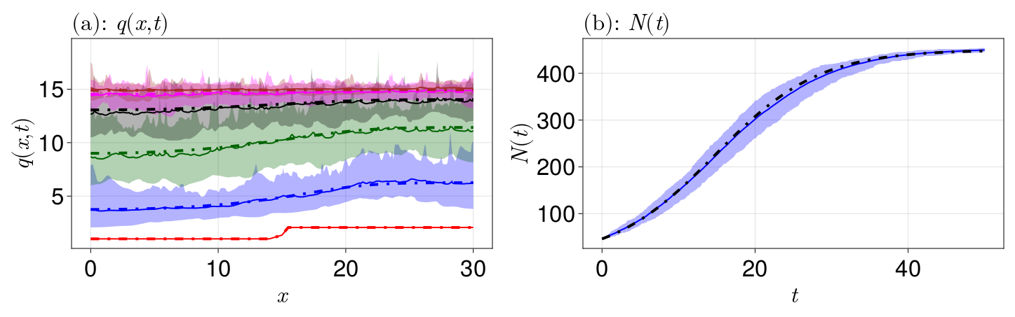

The confidence intervals are shown in the shaded regions, with the mean values given by a solid curve. We see that the continuum limit is a good match for the mean behaviour of both $q(x, t)$ and $N(t)$. The density $q(x, t)$ reaches a steady state with $q(x, t) \to 15$ as $t \to \infty$ for each $x$, which we expect given the cell carrying capacity density $K = 15$. If we had used e.g. a constant proliferation law $G(\delta) = \beta$, we would see growth indefinitely, so the logistic law is especially nice for this reason. The cell numbers reach a limit around $450$, which makes sense since $\int_0^{30} K\,\mathrm dx = 30K = 450$.

Example IV: Moving boundary, with proliferation

Now let us consider proliferation with a moving boundary.

using EpithelialDynamics1D, OrdinaryDiffEq
force_law = (δ, p) -> p.k * (p.s - δ)
force_law_parameters = (k=10.0, s=1)
proliferation_law = (δ, p) -> p.β *(one(δ) - inv(p.K * δ))
proliferation_law_parameters = (β=0.15, K=15.0)
proliferation_period = 1e-2
final_time = 30.0
damping_constant = 1.0
initial_condition = [LinRange(0, 15, 16); LinRange(15,30, 32)] |> unique!
prob = CellProblem(;
    force_law,
    force_law_parameters,
    proliferation_law,
    proliferation_law_parameters,
    proliferation_period,
    final_time,
    damping_constant,
    initial_condition,
    fix_right=false)
ens_prob = EnsembleProblem(prob)
sol = solve(ens_prob, Tsit5(); trajectories=50, saveat=001)

The continuum limit is the same as it was in Example II, except now the PDE is the one given in Example III. We construct this continuum limit as follows, noting again that MovingBoundaryProblems1D.jl solves the moving boundary problem:

using LinearSolve
mb_prob = continuum_limit(prob, 1000; proliferation=true)
mb_sol = solve(mb_prob, TRBDF2(linsolve=KLUFactorization()), saveat=0.01)

As in Example III, we can compute statistics from our ensemble solutions, as well as the corresponding values from the continuum limit:

(; q, r, means, lowers, uppers, knots) =node_densities(sol)
N, N_means, N_lowers, N_uppers = cell_numbers(sol)
L, L_means, L_lowers, L_uppers = leading_edge(sol)
pde_N = map(eachindex(mb_sol)) do i
    integrate_pde(mb_sol, i)
end
pde_L = map(mb_sol) do u
    u[end]
end

Let's now plot these results.

using CairoMakie
fig = Figure(fontsize=33)
colors = (:red, :blue, :darkgreen,:black, :magenta, :brown)
plot_idx = (1, 1001, 2001, 3001,4001, 5001)
ax = Axis(fig[1, 1], xlabel=L"x",ylabel=L"q(x, t)",
    title=L"(a): $q(x, t)$",titlealign=:left,
    width=600, height=300)
[band!(ax, knots[i], lowers[i],uppers[i], color=(colors[j], 0.3))for (j, i) in enumerate(plot_idx)]
[lines!(ax, knots[i], means[i],color=colors[j], linewidth=2) for(j, i) in enumerate(plot_idx)]
@views [lines!(ax, mb_sol.u[i][end] * mb_prob.geometry.mesh_points,mb_sol.u[i][begin:(end-1)],color=colors[j], linewidth=4,linestyle=:dashdot) for (j, i) in enumerate(plot_idx)]
ax = Axis(fig[1, 2], xlabel=L"t",ylabel=L"N(t)",
    title=L"(b): $N(t)$",titlealign=:left,
    width=600, height=300)
band!(ax, mb_sol.t, N_lowers,N_uppers, color=(:blue, 0.3))
lines!(ax, mb_sol.t, N_means,color=:blue, linewidth=2)
lines!(ax, mb_sol.t, pde_N,color=:black, linewidth=4,linestyle=:dashdot)
ax = Axis(fig[1, 3], xlabel=L"t",ylabel=L"L(t)",
    title=L"(c): $L(t)$",titlealign=:left,
    width=600, height=300)
band!(ax, mb_sol.t, L_lowers,L_uppers, color=(:blue, 0.3))
lines!(ax, mb_sol.t, L_means,color=:blue, linewidth=2)
lines!(ax, mb_sol.t, pde_L,color=:black, linewidth=4,linestyle=:dashdot)
resize_to_layout!(fig)

Once again, the continuum limit is a great match.