Example II: Logistic ordinary differential equation
The following example comes from the first case study of Simpson and Maclaren (2022). First, load the packages we'll be using:
using Random
using ProfileLikelihood
using Optimization
using OrdinaryDiffEq
using CairoMakie
using OptimizationNLopt
using Test
using StableRNGs
Let us consider the logistic ordinary differential equation (ODE). For ODEs, our treatment is as follows: Let us have some ODE $\mathrm dy/\mathrm dt = f(y, t; \boldsymbol \theta)$ for some parameters $\boldsymbol\theta$ of interest. We will suppose that we have some data $y_i^o$ at time $t_i$, $i=1,\ldots,n$, with initial condition $y_0^o$ at time $t_0=0$, which we model according to a normal distribution $y_i^o \mid \boldsymbol \theta \sim \mathcal N(y_i(\boldsymbol \theta), \sigma^2)$, $i=0,1,\ldots,n$, where $y_i$ is a solution of the ODE at time $t_i$. This defines a likelihood that we can use for estimating the parameters.
Let us now proceed with our example. We are considering $\mathrm du/\mathrm dt = \lambda u(1-u/K)$, $u(0)=u_0$, and our interest is in estimating $(\lambda, K, u_0)$, we will fix the standard deviation of the noise, $\sigma$, at $\sigma=10$. Note that the exact solution to this ODE is $u(t) = Ku_0/[(K-u_0)\mathrm{e}^{-\lambda t} + u_0]$.
Data generation and setting up the problem
The first step is to generate the data.
using OrdinaryDiffEq, Random, StableRNGs
λ = 0.01
K = 100.0
u₀ = 10.0
t = 0:100:1000
σ = 10.0
@inline function ode_fnc(u, p, t)
    λ, K = p
    du = λ * u * (1 - u / K)
    return du
end
# Initial data is obtained by solving the ODE
tspan = extrema(t)
p = (λ, K)
prob = ODEProblem(ode_fnc, u₀, tspan, p)
sol = solve(prob, Rosenbrock23(), saveat=t)
rng = StableRNG(123)
uᵒ = sol.u + σ * randn(rng, length(t))
Now having our data, we define the likelihood function.
function loglik_fnc2(θ, data, integrator)
    λ, K, u₀ = θ
    uᵒ, σ = data
    integrator.p[1] = λ
    integrator.p[2] = K
    reinit!(integrator, u₀)
    solve!(integrator)
    return gaussian_loglikelihood(uᵒ, integrator.sol.u, σ, length(uᵒ))
end
Now we can define our problem. We constrain the problem so that $0 \leq \lambda \leq 0.05$, $50 \leq K \leq 150$, and $0 \leq u_0 \leq 50$.
lb = [0.0, 50.0, 0.0] # λ, K, u₀
ub = [0.05, 150.0, 50.0]
θ₀ = [λ, K, u₀]
syms = [:λ, :K, :u₀]
prob = LikelihoodProblem(
    loglik_fnc2, θ₀, ode_fnc, u₀, maximum(t); # Note that u₀ is just a placeholder IC in this case since we are estimating it
    syms=syms,
    data=(uᵒ, σ),
    ode_parameters=[1.0, 1.0], # temp values for [λ, K]
    ode_kwargs=(verbose=false, saveat=t),
    f_kwargs=(adtype=Optimization.AutoFiniteDiff(),),
    prob_kwargs=(lb=lb, ub=ub),
    ode_alg=Rosenbrock23()
)
Parameter estimation
Now we find the MLEs.
using OptimizationNLopt
@time sol = mle(prob, NLopt.LD_LBFGS)
LikelihoodSolution. retcode: Success
Maximum likelihood: -37.85651768034309
Maximum likelihood estimates: 3-element Vector{Float64}
     λ: 0.011487034703855741
     K: 92.91981958228756
     u₀: 7.32571300295812
We can now profile.
prof = profile(prob, sol; alg=NLopt.LN_NELDERMEAD, parallel=false)
ProfileLikelihoodSolution. MLE retcode: Success
Confidence intervals:
     95.0% CI for λ: (0.0071020420981672125, 0.0203926571982326)
     95.0% CI for K: (84.8643752054692, 101.47721534417298)
     95.0% CI for u₀: (0.8563282019943417, 19.058369692049276)
@test λ ∈ get_confidence_intervals(prof, :λ)
@test K ∈ prof.confidence_intervals[2]
@test u₀ ∈ get_confidence_intervals(prof, 3)We can visualise as we did before:
using CairoMakie
fig = plot_profiles(prof;
    latex_names=[L"\lambda", L"K", L"u_0"],
    show_mles=true,
    shade_ci=true,
    nrow=1,
    ncol=3,
    true_vals=[λ, K, u₀],
    fig_kwargs=(fontsize=41,),
    axis_kwargs=(width=600, height=300))
resize_to_layout!(fig)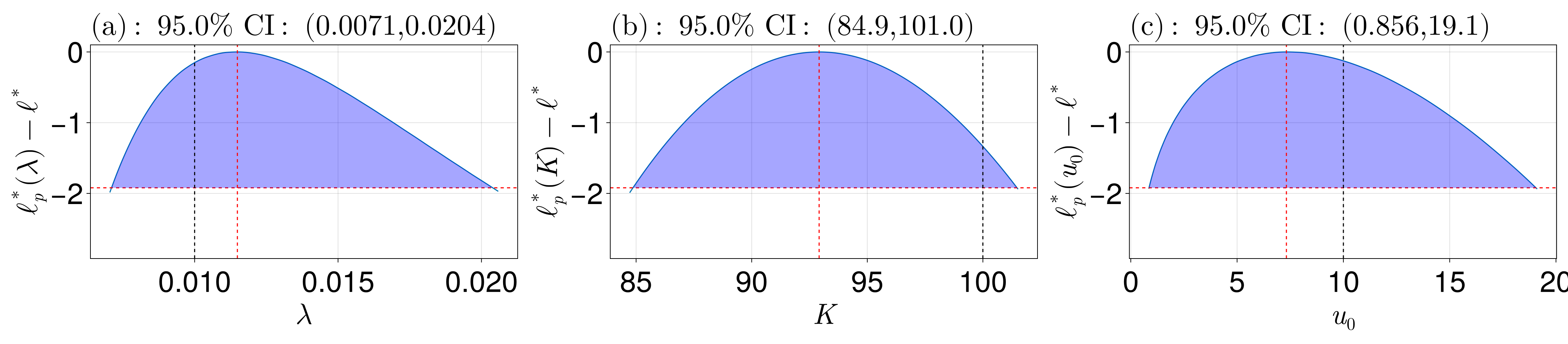
Prediction intervals
Let us now use these results to compute prediction intervals for $u(t)$. Following Simpson and Maclaren (2022), the idea is to use the profile likelihood to construct another profile likelihood, called the profile-wise profile likelihood, that allows us to obtain prediction intervals for some prediction function $q(\boldsymbol \theta)$. More detail is given in the mathematical details section.
The first step is to define a function $q(\boldsymbol\theta)$ that comptues our prediction given some parameters $\boldsymbol\theta$. The function in this case is simply:
function prediction_function(θ, data)
    λ, K, u₀ = θ
    t = data
    prob = ODEProblem(ode_fnc, u₀, extrema(t), (λ, K))
    sol = solve(prob, Rosenbrock23(), saveat=t)
    return sol.u
end
Note that the second argument data allows for extra parameters to be passed. To now obtain prediction intervals for sol.u, for each t, we define a large grid for t and use get_prediction_intervals:
t_many_pts = LinRange(extrema(t)..., 1000)
parameter_wise, union_intervals, all_curves, param_range =
    get_prediction_intervals(prediction_function, prof,
        t_many_pts; parallel=true)
# t_many_pts is the `data` argument, it doesn't have to be time for other problems
This function get_prediction_intervals has four outputs:
parameter_wise: These are prediction intervals for the prediction at each point $t$, coming from the profile likelihood of each respective parameter:
julia> parameter_wise
Dict{Int, Vector{ProfileLikelihood.ConfidenceInterval{Float64, Float64}}} with 3 entries:
  2 => [ConfidenceInterval{Float64, Float64}(6.36401, 9.76387, 0.95), ConfidenceInterval{Float64, Float64}(6.4406, 9.84797, 0.95), ConfidenceInterval{Float64, Float64}(6.51…
  3 => [ConfidenceInterval{Float64, Float64}(0.856328, 19.0584, 0.95), ConfidenceInterval{Float64, Float64}(0.87343, 19.1744, 0.95), ConfidenceInterval{Float64, Float64}(0.…
  1 => [ConfidenceInterval{Float64, Float64}(0.960745, 17.3585, 0.95), ConfidenceInterval{Float64, Float64}(0.980345, 17.4599, 0.95), ConfidenceInterval{Float64, Float64}(1…
For example, parameter_wise[1] comes from varying $\lambda$, with the parameters $K$ and $u_0$ coming from optimising the likelihood function with $\lambda$ fixed.
union_intervals: These are prediction intervals at each point $t$ coming from taking the union of the intervals from the corresponding elements ofparameter_wise.all_curves: The intervals come from taking extrema over many curves. This is aDictmapping parameter indices to the curves that were used, withall_curves[i][j]being the set of curves for theith parameter (e.g.i=1is for $\lambda$) and thejth parameter.param_range: The curves come from evaluating the prediction function between the bounds of the confidence intervals for each parameter, and this output gives the parameters used, so that e.g.all_curves[i][j]usesparam_range[i][j]for the value of theith parameter.
Let us now use these outputs to visualise the prediction intervals. First, let us extract the solution with the true parameter values and with the MLEs.
exact_soln = prediction_function([λ, K, u₀], t_many_pts)
mle_soln = prediction_function(get_mle(sol), t_many_pts)
Now let us plot the prediction intervals coming from each parameter, and from the union of all intervals (not shown yet, see below).
fig = Figure(fontsize=38)
alp = join('a':'z')
latex_names = [L"\lambda", L"K", L"u_0"]
for i in 1:3
    ax = Axis(fig[i < 3 ? 1 : 2, i < 3 ? i : 1], title=L"(%$(alp[i])): Profile-wise PI for %$(latex_names[i])",
        titlealign=:left, width=600, height=300)
    [lines!(ax, t_many_pts, all_curves[i][:, j], color=:grey) for j in eachindex(param_range[1])]
    lines!(ax, t_many_pts, exact_soln, color=:red)
    lines!(ax, t_many_pts, mle_soln, color=:blue, linestyle=:dash)
    lines!(ax, t_many_pts, getindex.(parameter_wise[i], 1), color=:black, linewidth=3)
    lines!(ax, t_many_pts, getindex.(parameter_wise[i], 2), color=:black, linewidth=3)
end
ax = Axis(fig[2, 2], title=L"(d):$ $ Union of all intervals",
    titlealign=:left, width=600, height=300)
band!(ax, t_many_pts, getindex.(union_intervals, 1), getindex.(union_intervals, 2), color=:grey)
lines!(ax, t_many_pts, getindex.(union_intervals, 1), color=:black, linewidth=3)
lines!(ax, t_many_pts, getindex.(union_intervals, 2), color=:black, linewidth=3)
lines!(ax, t_many_pts, exact_soln, color=:red)
lines!(ax, t_many_pts, mle_soln, color=:blue, linestyle=:dash)
To now assess the coverage of these intervals, we want to compare them to the interval coming from the full likelihood. We find this interval by taking a large number of parameters, and finding all of them for which the normalised log-likelihood exceeds the threshold $-1.92$. We then take the parameters that give a value exceeding this threshold, compute the prediction function at these values, and then take the extrema. The code below uses the function grid_search that evaluates the function at many points, and we describe this function in more detail in the next example.
lb = get_lower_bounds(prob)
ub = get_upper_bounds(prob)
N = 1e5
grid = [[lb[i] + (ub[i] - lb[i]) * rand() for _ in 1:N] for i in 1:3]
grid = permutedims(reduce(hcat, grid), (2, 1))
ig = IrregularGrid(lb, ub, grid)
gs, lik_vals = grid_search(prob, ig; parallel=Val(true), save_vals=Val(true))
lik_vals .-= get_maximum(sol) # normalised
feasible_idx = findall(lik_vals .> ProfileLikelihood.get_chisq_threshold(0.95)) # values in the confidence region
parameter_evals = grid[:, feasible_idx]
q = [prediction_function(θ, t_many_pts) for θ in eachcol(parameter_evals)]
q_mat = reduce(hcat, q)
q_lwr = minimum(q_mat; dims=2) |> vec
q_upr = maximum(q_mat; dims=2) |> vec
lines!(ax, t_many_pts, q_lwr, color=:magenta, linewidth=3)
lines!(ax, t_many_pts, q_upr, color=:magenta, linewidth=3)
resize_to_layout!(fig)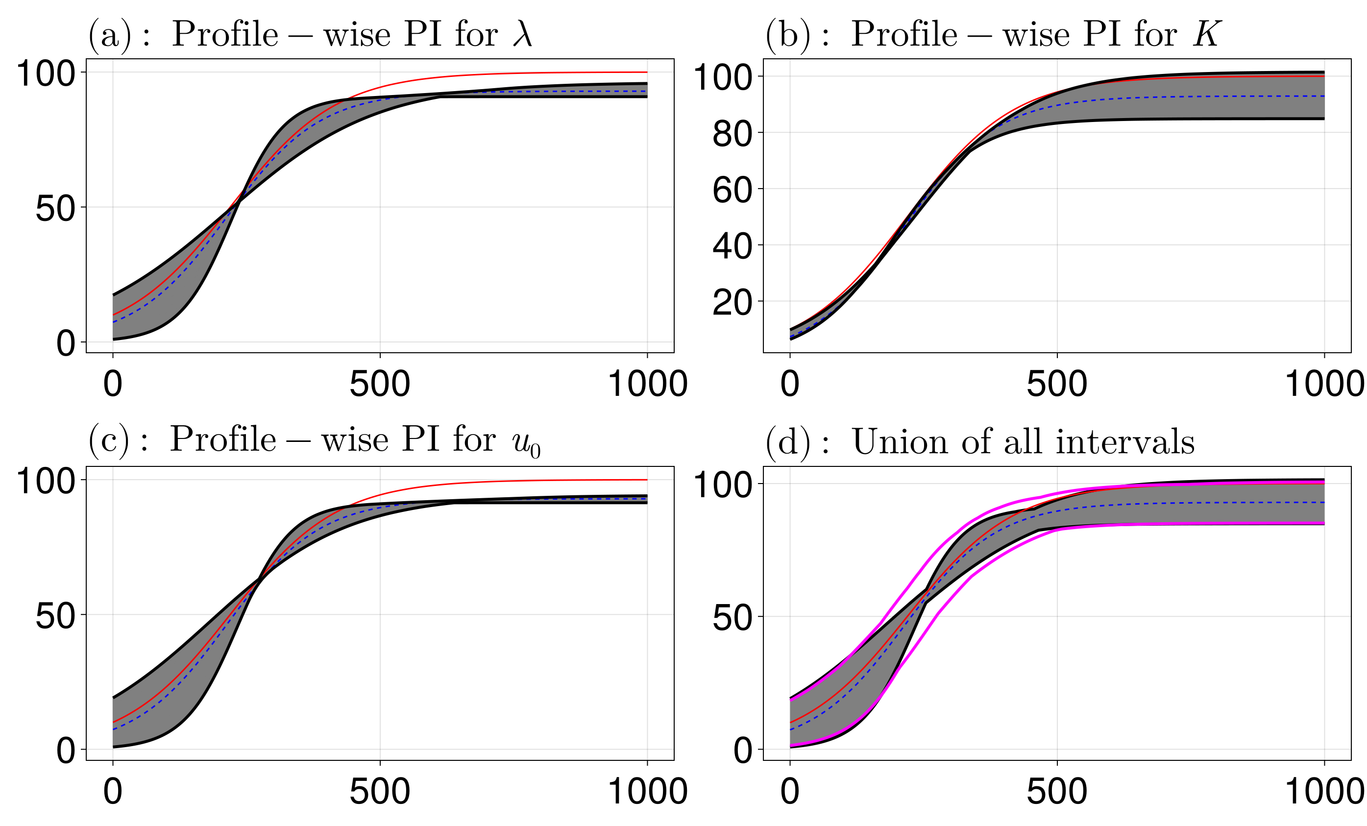
The first plot shows that the profile-wise prediction interval for $\lambda$ is quite large when $t$ is small, and then small for large time. This makes sense since the large time solution is independent of $\lambda$ (the large time solution is $u_s(t)=K$). For $K$, we see that the profile-wise interval only becomes large for large time, which again makes sense. For $u_0$ we see similar behaviour as for $\lambda$. Finally, taking the union over all the intervals, as is done in (d), shows that we fully enclose the solution coming from the MLE, as well as the true curve. The magenta curve shows the results from the full likelihood function, and is reasonably close to the approximate interval obtained from the union.