Example I: Multiple linear regression
Let us start with a linear regression example. First, load the packages needed:
using ProfileLikelihood
using Random
using PreallocationTools
using Distributions
using CairoMakie
using LinearAlgebra
using Optimization
using OptimizationOptimJL
using Test
using StableRNGs
We perform a simulation study where we try and estimate the parameters in a regression of the form
\[y_i = \beta_0 + \beta_1x_{1i} + \beta_2x_{2i} + \beta_3x_{1i}x_{3i} + \varepsilon_i, \quad \varepsilon_i \sim \mathcal N(0, \sigma^2), \quad i=1,2,\ldots, n. \]
We also try and estimate $\sigma$.
Setting up the problem
Let us start by simulating the data:
using Random, Distributions, StableRNGs
rng = StableRNG(98871)
n = 600
β = [-1.0, 1.0, 0.5, 3.0]
σ = 0.05
x₁ = rand(rng, Uniform(-1, 1), n)
x₂ = rand(rng, Normal(1.0, 0.5), n)
X = hcat(ones(n), x₁, x₂, x₁ .* x₂)
ε = rand(rng, Normal(0.0, σ), n)
y = X * β + ε
The data y is now our noisy data. The likelihood function in this example is
\[\ell(\sigma, \boldsymbol \beta \mid \boldsymbol y) = -(n/2)\log(2\mathrm{\pi}\sigma^2) - (1/2\sigma^2)\sum_i (y_i - \beta_0 - \beta_1x_{1i} - \beta_2x_{2i} - \beta_3x_{1i}x_{2i})^2. \]
We now define our likelihood function. To allow for automatic differentiation, we use PreallocationTools.DiffCache to define our cache vectors.
sse = DiffCache(zeros(n))
β_cache = DiffCache(similar(β), 10)
dat = (y, X, sse, n, β_cache)
@inline function loglik_fnc(θ, data)
    σ, β₀, β₁, β₂, β₃ = θ
    y, X, sse, n, β = data
    _sse = get_tmp(sse, θ)
    _β = get_tmp(β, θ)
    _β[1] = β₀
    _β[2] = β₁
    _β[3] = β₂
    _β[4] = β₃
    ℓℓ = -0.5n * log(2π * σ^2)
    mul!(_sse, X, _β)
    for i in eachindex(y)
        ℓℓ = ℓℓ - 0.5 / σ^2 * (y[i] - _sse[i])^2
    end
    return ℓℓ
end
Now having defined our likelihood, we can define the likelihood problem. We let the problem be unconstrained, except for $\sigma > 0$. We start at the value $1$ for each parameter. To use automatic differentiation, we use Optimization.AutoForwardDiff for the adtype.
using Optimization
θ₀ = ones(5)
prob = LikelihoodProblem(loglik_fnc, θ₀;
    data=dat,
    f_kwargs=(adtype=Optimization.AutoForwardDiff(),),
    prob_kwargs=(
        lb=[0.0, -Inf, -Inf, -Inf, -Inf],
        ub=Inf * ones(5)
    ),
    syms=[:σ, :β₀, :β₁, :β₂, :β₃]
)
LikelihoodProblem. In-place: true
θ₀: 5-element Vector{Float64}
     σ: 1.0
     β₀: 1.0
     β₁: 1.0
     β₂: 1.0
     β₃: 1.0
Finding the MLEs
Now we can compute the MLEs.
using OptimizationOptimJL
sol = mle(prob, Optim.LBFGS())
LikelihoodSolution. retcode: Success
Maximum likelihood: 953.0592307643246
Maximum likelihood estimates: 5-element Vector{Float64}
     σ: 0.04942145761216433
     β₀: -1.003655020311133
     β₁: 0.9980076846106273
     β₂: 0.5030706527702703
     β₃: 2.9989096752667272
We can compare these MLEs to the true MLES $\hat{\beta} = (\boldsymbol X^{\mathsf T}\boldsymbol X)^{-1}\boldsymbol X^{\mathsf T}\boldsymbol y$ and $\hat\sigma^2 = (1/n_d)(\boldsymbol y - \boldsymbol X\boldsymbol \beta)^{\mathsf T}(\boldsymbol y - \boldsymbol X\boldsymbol \beta)$, where $n_d$ is the degrees of freedom, as follows (note the indexing):
using Test, LinearAlgebra
df = n - (length(β) + 1)
resids = y .- X * sol[2:5]
@test sol[2:5] ≈ inv(X' * X) * X' * y # sol[i] = sol.mle[i]
@test sol[:σ]^2 ≈ 1 / df * sum(resids .^ 2) atol = 1e-4 # symbol indexing
Profiling
We can now profile the results. In this case, since the problem has no bounds for some parameters we need to manually define the parameter bounds used for profiling. The function construct_profile_ranges is used for this. Note that we use parallel = true below to allow for multithreading, allowing multiple parameters to be profiled at the same time.
lb = [1e-12, -5.0, -5.0, -5.0, -5.0]
ub = [15.0, 15.0, 15.0, 15.0, 15.0]
resolutions = [600, 200, 200, 200, 200] # use many points for σ
param_ranges = construct_profile_ranges(sol, lb, ub, resolutions)
prof = profile(prob, sol; param_ranges, parallel=true)
ProfileLikelihoodSolution. MLE retcode: Success
Confidence intervals:
     95.0% CI for σ: (0.04675191495089245, 0.052360551143196946)
     95.0% CI for β₀: (-1.0121607844224445, -0.9951520336370397)
     95.0% CI for β₁: (0.9826173262148143, 1.0133977395553302)
     95.0% CI for β₂: (0.4954041345031461, 0.5107344459064201)
     95.0% CI for β₃: (2.9847775716187175, 3.013042187605372)
These confidence intervals can be compared to the true confidence intervals as follows, noting that the variance-covariance matrix for the $\beta_i$ coefficients is $\boldsymbol\Sigma = \sigma^2(\boldsymbol X^{\mathsf T}\boldsymbol X)^{-1}$ so that their confidence interval is $\hat\beta_i \pm 1.96\sqrt{\boldsymbol\Sigma_{ii}}$. Additionally, a confidence interval for $\sigma$ is $\sqrt{(\boldsymbol y - \boldsymbol X\boldsymbol \beta)^{\mathsf T}(\boldsymbol y - \boldsymbol X\boldsymbol \beta)}(1/\sqrt{\chi_{0.975, n_d}}, 1/\sqrt{\chi_{0.025, n_d}})$.
vcov_mat = sol[:σ]^2 * inv(X' * X)
for i in 1:4
    @test prof.confidence_intervals[i+1][1] ≈ sol.mle[i+1] - 1.96sqrt(vcov_mat[i, i]) atol = 1e-3
    @test prof.confidence_intervals[i+1][2] ≈ sol.mle[i+1] + 1.96sqrt(vcov_mat[i, i]) atol = 1e-3
end
rss = sum(resids .^ 2)
χ²_up = quantile(Chisq(df), 0.975)
χ²_lo = quantile(Chisq(df), 0.025)
σ_CI_exact = sqrt.(rss ./ (χ²_up, χ²_lo))
@test get_confidence_intervals(prof, :σ).lower ≈ σ_CI_exact[1] atol = 1e-3
@test ProfileLikelihood.get_upper(get_confidence_intervals(prof, :σ)) ≈ σ_CI_exact[2] atol = 1e-3
You can use prof to view a single parameter's results, e.g.
julia> prof[:β₂] # This is a ProfileLikelihoodSolutionView
Profile likelihood for parameter β₂. MLE retcode: Success
MLE: 0.5030706527702703
95.0% CI for β₂: (0.4954041345031461, 0.5107344459064201)
You can also evaluate the profile at a point inside its confidence interval. (If you want to evaluate outside the confidence interval, you need to use a non-Throw extrap in the profile function's keyword argument [see also Interpolations.jl].) The following are all the same, evaluating the profile for $\beta_2$ at $\beta_2=0.5$:
prof[:β₂](0.50)
prof(0.50, :β₂)
prof(0.50, 4)
Visualisation
We can now also visualise the results. In the plot below, the red line is at the threshold for the confidence region, so that the parameters between these values define the confidence interval. The red lines are at the MLEs, and the black lines are at the true values.
using CairoMakie
fig = plot_profiles(prof;
    latex_names=[L"\sigma", L"\beta_0", L"\beta_1", L"\beta_2", L"\beta_3"], # default names would be of the form θᵢ
    show_mles=true,
    shade_ci=true,
    true_vals=[σ, β...],
    fig_kwargs=(fontsize=41,),
    axis_kwargs=(width=600, height=300))
xlims!(fig.content[1], 0.045, 0.055) # fix the ranges
xlims!(fig.content[2], -1.025, -0.975)
xlims!(fig.content[4], 0.475, 0.525)
resize_to_layout!(fig)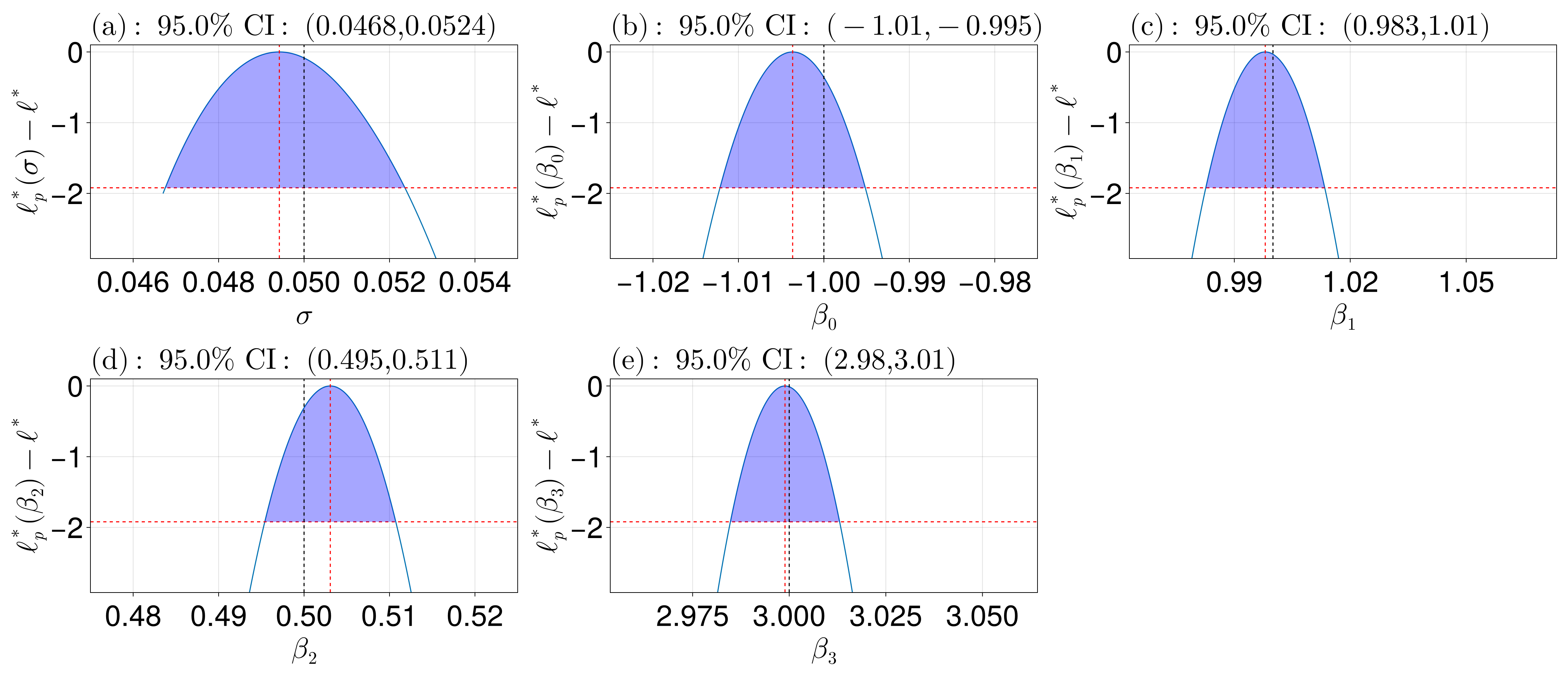
You could also plot individual or specific parameters:
plot_profiles(prof, [1, 3]) # plot σ and β₁
plot_profiles(prof, [:σ, :β₁, :β₃]) # can use symbols
plot_profiles(prof, 1) # can just provide an integer
plot_profiles(prof, :β₂) # symbols work