Example IV: Lotka-Volterra ODE and computing bivarate profile likelihoods

This example comes from the second case study of Simpson and Maclaren (2022). First, load the packages we'll be using:

using Random
using Optimization
using OrdinaryDiffEq
using CairoMakie
using ProfileLikelihood
using OptimizationNLopt
using StableRNGs

In this example, we will be considering the Lotka-Volterra ODE. We show how bivariate profiles can be computed, along with prediction intervals from a bivariate profile. The Lotka-Volterra ODE is given by

\[\begin{align*} \frac{\mathrm da(t)}{\mathrm dt} &= \alpha a(t) - a(t)b(t), \\ \frac{\mathrm db(t)}{\mathrm dt} &= \beta a(t)b(t)-b(t), \end{align*}\]

and we suppose that $a(0) = a_0$ and $b(0) = b_0$. For this problem, we are interested in estimating $\boldsymbol = (\alpha,\beta,a_0,b_0)$. We suppose that we have measures of the prey and predicator populations, given respectively by $a(t)$ and $b(t)$, at times $t_i$, $i=1,\ldots,m$. Letting $a_i^ o = a(t_i)$ and $b_i^o = b(t_i)$, $i=1,\ldots,m$, this means that we have the time series $\{(a_i^o, b_i^o)\}_{i=1}^m$. Moreover, just as we did in the logistic ODE example, we suppose that the data $(a_i^o, b_i^o)$ are normally distributed about the solution curve $\boldsymbol z(t; \boldsymbol\theta) = (a(t; \boldsymbol \theta), b(t; \boldsymbol \theta))$. In particular, letting $\boldsymbol z_i(\boldsymbol \theta)$ denote the value of $(a(t_i; \boldsymbol\theta), b(t_i; \boldsymbol \theta))$ at $t=t_i$, we are supposing that

\[(a_i^o, b_i^o) \sim \mathcal N\left(\boldsymbol z_i(\boldsymbol \theta), \sigma^2 \boldsymbol I\right), \quad i=1,2,\ldots,m,\]

and this is what defines our likelihood ($\boldsymbol I$ is the $2$-square identity matrix). We use values $0 \leq t \leq 7$ for estimation, and predict on $0 \leq t \leq 10$.

Data generation and setting up the problem

As usual, the first step in this example is generating the data.

using OrdinaryDiffEq, Random, StableRNGs

## Step 1: Generate the data and define the likelihood
α = 0.9
β = 1.1
a₀ = 0.8
b₀ = 0.3
σ = 0.2
t = LinRange(0, 10, 21)
@inline function ode_fnc!(du, u, p, t) 
    α, β = p
    a, b = u
    du[1] = α * a - a * b
    du[2] = β * a * b - b
    return nothing
end
# Initial data is obtained by solving the ODE 
tspan = extrema(t)
p = [α, β]
u₀ = [a₀, b₀]
prob = ODEProblem(ode_fnc!, u₀, tspan, p)
sol = solve(prob, Rosenbrock23(), saveat=t)
rng = StableRNG(2828881)
noise_vec = [σ * randn(rng, 2) for _ in eachindex(t)]
uᵒ = sol.u .+ noise_vec

We now define the likelihood function.

function loglik_fnc2(θ::AbstractVector{T}, data, integrator) where {T}
    α, β, a₀, b₀ = θ
    uᵒ, σ, u₀, n = data
    integrator.p[1] = α
    integrator.p[2] = β
    u₀[1] = a₀
    u₀[2] = b₀
    reinit!(integrator, u₀)
    solve!(integrator)
    ℓ = zero(T)
    for i in 1:n
        âᵒ = integrator.sol.u[i][1]
        b̂ᵒ = integrator.sol.u[i][2]
        aᵒ = uᵒ[i][1]
        bᵒ = uᵒ[i][2]
        ℓ = ℓ - 0.5log(2π * σ^2) - 0.5(âᵒ - aᵒ)^2 / σ^2
        ℓ = ℓ - 0.5log(2π * σ^2) - 0.5(b̂ᵒ - bᵒ)^2 / σ^2
    end
    return ℓ
end

Now we define our problem, constraining the parameters so that $0.7 \leq \alpha \leq 1.2$, $0.7 \leq \beta \leq 1.4$, $0.5 \leq a_0 \leq 1.2$, and $0.1 \leq b_0 \leq 0.5$.

using Optimization, OrdinaryDiffEq, ProfileLikelihood
lb = [0.7, 0.7, 0.5, 0.1]
ub = [1.2, 1.4, 1.2, 0.5]
θ₀ = [0.75, 1.23, 0.76, 0.292]
syms = [:α, :β, :a₀, :b₀]
u₀_cache = zeros(2)
n = findlast(t .≤ 7) # Using t ≤ 7 for estimation
prob = LikelihoodProblem(
    loglik_fnc2, θ₀, ode_fnc!, u₀, tspan;
    syms=syms,
    data=(uᵒ, σ, u₀_cache, n),
    ode_parameters=[1.0, 1.0],
    ode_kwargs=(verbose=false, saveat=t),
    prob_kwargs = (lb=lb, ub=ub),
    ode_alg=Rosenbrock23()
)

LikelihoodProblem. In-place: true
θ₀: 4-element Vector{Float64}
     α: 0.75
     β: 1.23
     a₀: 0.76
     b₀: 0.292

Parameter estimation

Let us now proceed as usual, computing the MLEs and obtaining the profiles.

julia> using OptimizationNLopt
julia> @time sol = mle(prob, NLopt.LN_NELDERMEAD)
  0.022843 seconds (266.05 k allocations: 10.547 MiB)
LikelihoodSolution. retcode: Success
Maximum likelihood: 7.083346779938254
Maximum likelihood estimates: 4-element Vector{Float64}
     α: 0.8798816617243157
     β: 1.123199229773868
     a₀: 0.860737893924461
     b₀: 0.3320559683543075

julia> @time prof = profile(prob, sol; parallel=true)
  9.348295 seconds (96.71 M allocations: 3.830 GiB, 3.52% gc time)
ProfileLikelihoodSolution. MLE retcode: Success
Confidence intervals:
     95.0% CI for α: (0.7655588053712551, 0.9947597721255612)
     95.0% CI for β: (1.014685357334102, 1.2569672111855281)
     95.0% CI for a₀: (0.7315323205415538, 0.9964615701946258)
     95.0% CI for b₀: (0.24194969128552055, 0.43338299417186515)

Now plotting the profiles:

using CairoMakie
fig = plot_profiles(prof;
    latex_names=[L"\alpha", L"\beta", L"a_0", L"b_0"],
    show_mles=true,
    shade_ci=true,
    nrow=2,
    ncol=2,
    true_vals=[α, β, a₀, b₀])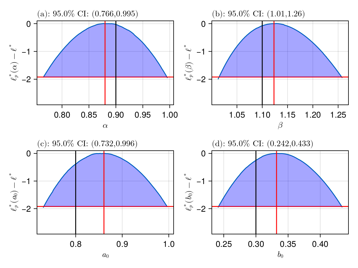

Bivariate profiles

In all the examples thus far, we have only considered univariate profiles. We also provide a method for computing bivariate profiles through the bivariate_profile function. In this function instead of providing a set of integers for the parameters to profile, we provide tuples of integers (or symbols). Let's compute the bivariate profiles for all pairs. In the code below, resolution=25 means we define 25 layers between the MLE and the bounds for each parameter (see the implementation details section in the sidebar for a definition of a layer). Setting outer_layers=10 means that we go out 10 layers even after finding the complete confidence region.

param_pairs = ((:α, :β), (:α, :a₀), (:α, :b₀),
    (:β, :a₀), (:β, :b₀),
    (:a₀, :b₀)) # Same as param_pairs = ((1, 2), (1, 3), (1, 4), (2, 3), (2, 4), (3, 4))
@time prof_2 = bivariate_profile(prob, sol, param_pairs; parallel=true, resolution=25, outer_layers=10) 
# Multithreading highly recommended for bivariate profiles - even a resolution of 25 is an upper bound of 2,601 optimisation problems for each pair (in general, this number is 4N(N+1) + 1 for a resolution of N).

255.794233 seconds (1.15 G allocations: 45.774 GiB, 2.00% gc time, 2.20% compilation time)
BivariateProfileLikelihoodSolution. MLE retcode: Success
Profile info:
     (β, b₀): 25 layers. Bbox for 95.0% CR: [0.9910523784900991, 1.29477713384572] × [0.21992309825215978, 0.45954937571653703]
     (α, β): 25 layers. Bbox for 95.0% CR: [0.7357005284921787, 1.0221575680079797] × [0.991123194005582, 1.2949721520687736]
     (α, a₀): 25 layers. Bbox for 95.0% CR: [0.7357619449614752, 1.0219994350896653] × [0.702688464342064, 1.0333477627025405]
     (a₀, b₀): 25 layers. Bbox for 95.0% CR: [0.7026997627224284, 1.0333698932787927] × [0.21999696665137455, 0.459589626124184]
     (α, b₀): 25 layers. Bbox for 95.0% CR: [0.7357403217306449, 1.0221076705696055] × [0.21999378985874352, 0.45959053842574044]
     (β, a₀): 25 layers. Bbox for 95.0% CR: [0.9912086964720968, 1.2949252238744442] × [0.7026534659606257, 1.0329841074487238]

To plot these profiles, we can use plot_profiles. These plots usually take a bit more work than the univariate case. Let's first show a poor plot. We specify xlims and ylims to match Simpson and Maclaren (2022).

fig_2 = plot_profiles(prof_2, param_pairs; # param_pairs not needed, but this ensures we get the correct order
    latex_names=[L"\alpha", L"\beta", L"a_0", L"b_0"],
    show_mles=true,
    nrow=3,
    ncol=2,
    true_vals=[α, β, a₀, b₀],
    xlim_tuples=[(0.5, 1.5), (0.5, 1.5), (0.5, 1.5), (0.7, 1.3), (0.7, 1.3), (0.5, 1.1)],
    ylim_tuples=[(0.5, 1.5), (0.5, 1.05), (0.1, 0.5), (0.5, 1.05), (0.1, 0.5), (0.1, 0.5)],
    fig_kwargs=(fontsize=17,))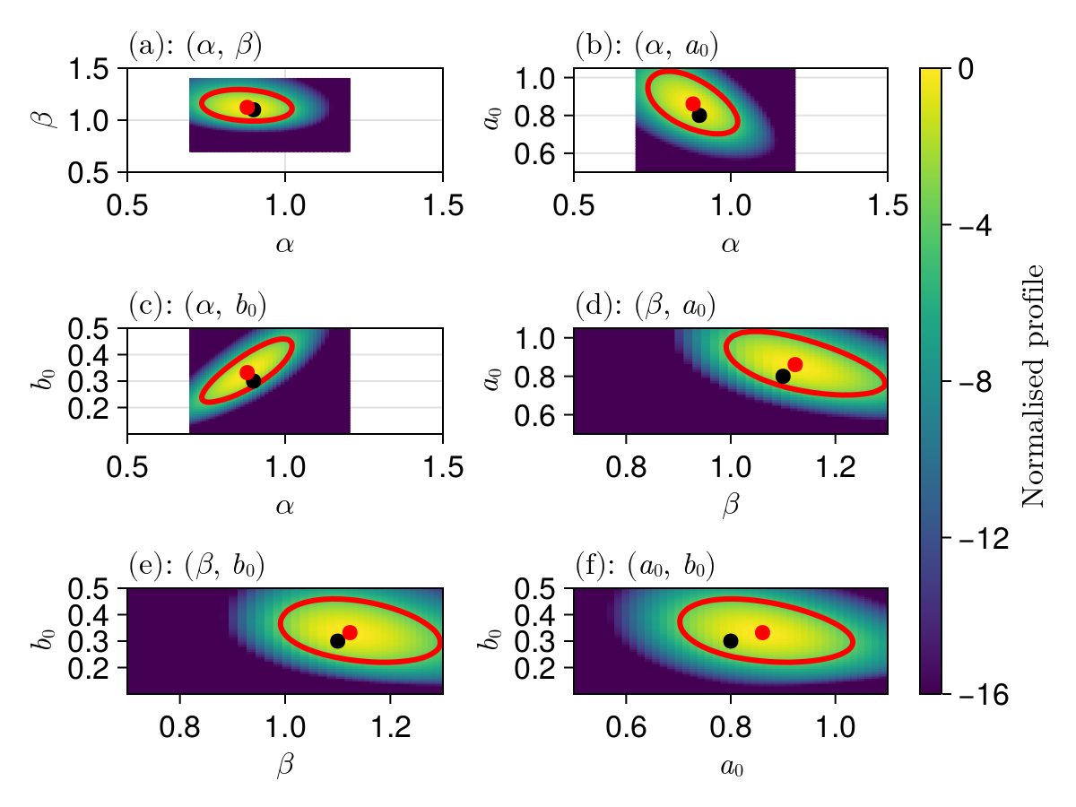

In these plots, the red boundaries mark the confidence region's boundary, the red dot shows the MLE, and the black dots are the true values. There are two issues with these plots:

The plots are quite pixelated due to the low resolution.
The plots don't fill out the entire axis.

These two issues can be resolved using the interpolant defined from the original data. Setting interpolant = true resolves these two problems. (If we also had a poor quality confidence region, you could also set smooth_confidence_boundary = true.)

fig_3 = plot_profiles(prof_2, param_pairs;
    latex_names=[L"\alpha", L"\beta", L"a_0", L"b_0"],
    show_mles=true,
    nrow=3,
    ncol=2,
    true_vals=[α, β, a₀, b₀],
    interpolation=true,
    xlim_tuples=[(0.5, 1.5), (0.5, 1.5), (0.5, 1.5), (0.7, 1.3), (0.7, 1.3), (0.5, 1.1)],
    ylim_tuples=[(0.5, 1.5), (0.5, 1.05), (0.1, 0.5), (0.5, 1.05), (0.1, 0.5), (0.1, 0.5)],
    fig_kwargs=(fontsize=17,))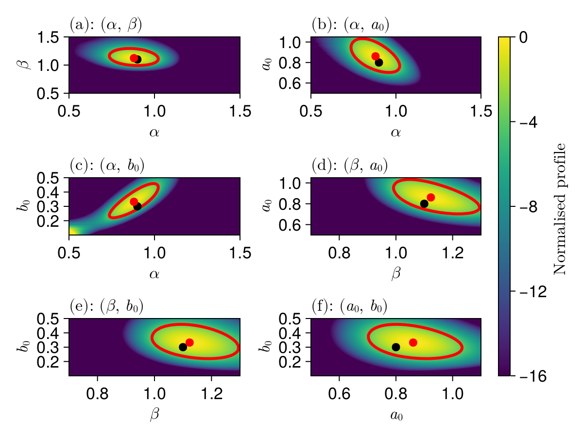

Prediction intervals

Let's now proceed with finding prediction intervals. We first find the prediction intervals using our univariate results. We use the in-place version of a prediction function:

function prediction_function!(q, θ::AbstractVector{T}, data) where {T}
    α, β, a₀, b₀ = θ
    t, a_idx, b_idx = data
    prob = ODEProblem(ODEFunction(ode_fnc!, syms=(:a, :b)), [a₀, b₀], extrema(t), (α, β))
    sol = solve(prob, Rosenbrock23(), saveat=t)
    q[a_idx] .= sol[:a]
    q[b_idx] .= sol[:b]
    return nothing
end
t_many_pts = LinRange(extrema(t)..., 1000)
a_idx = 1:1000
b_idx = 1001:2000
pred_data = (t_many_pts, a_idx, b_idx)
q_prototype = zeros(2000)
individual_intervals, union_intervals, q_vals, param_ranges =
    get_prediction_intervals(prediction_function!, prof, pred_data; parallel=true,
        q_prototype)

Now we plot these results, plotting the individual intervals as well as the union intervals. As in Example II, we also look at the intervals from the full likelihood.

# Evaluate the exact and MLE solutions
exact_soln = zeros(2000)
mle_soln = zeros(2000)
prediction_function!(exact_soln, [α, β, a₀, b₀], pred_data)
prediction_function!(mle_soln, get_mle(sol), pred_data)

# Plot the parameter-wise intervals 
fig = Figure(fontsize=38, size=(2935.488f0, 1392.64404f0))
alp = [['a', 'b', 'e', 'f'], ['c', 'd', 'g', 'h']]
latex_names = [L"\alpha", L"\beta", L"a_0", L"b_0"]
for (k, idx) in enumerate((a_idx, b_idx))
    for i in 1:4
        ax = Axis(fig[i < 3 ? 1 : 2, mod1(i, 2)+(k==2)*2], title=L"(%$(alp[k][i])): Profile-wise PI for %$(latex_names[i])",
            titlealign=:left, width=600, height=300, xlabel=L"t", ylabel=k == 1 ? L"a(t)" : L"b(t)")
        vlines!(ax, [7.0], color=:purple, linestyle=:dash, linewidth=2)
        lines!(ax, t_many_pts, exact_soln[idx], color=:red, linewidth=3)
        lines!(ax, t_many_pts, mle_soln[idx], color=:blue, linestyle=:dash, linewidth=3)
        lines!(ax, t_many_pts, getindex.(individual_intervals[i], 1)[idx], color=:black, linewidth=3)
        lines!(ax, t_many_pts, getindex.(individual_intervals[i], 2)[idx], color=:black, linewidth=3)
        band!(ax, t_many_pts, getindex.(individual_intervals[i], 1)[idx], getindex.(individual_intervals[i], 2)[idx], color=(:grey, 0.35))
    end
end

# Plot the union intervals
a_ax = Axis(fig[3, 1:2], title=L"(i):$ $ Union of all intervals",
    titlealign=:left, width=1200, height=300, xlabel=L"t", ylabel=L"a(t)")
b_ax = Axis(fig[3, 3:4], title=L"(j):$ $ Union of all intervals",
    titlealign=:left, width=1200, height=300, xlabel=L"t", ylabel=L"b(t)")
_ax = (a_ax, b_ax)
for (k, idx) in enumerate((a_idx, b_idx))
    band!(_ax[k], t_many_pts, getindex.(union_intervals, 1)[idx], getindex.(union_intervals, 2)[idx], color=(:grey, 0.35))
    lines!(_ax[k], t_many_pts, getindex.(union_intervals, 1)[idx], color=:black, linewidth=3)
    lines!(_ax[k], t_many_pts, getindex.(union_intervals, 2)[idx], color=:black, linewidth=3)
    lines!(_ax[k], t_many_pts, exact_soln[idx], color=:red, linewidth=3)
    lines!(_ax[k], t_many_pts, mle_soln[idx], color=:blue, linestyle=:dash, linewidth=3)
    vlines!(_ax[k], [7.0], color=:purple, linestyle=:dash, linewidth=2)
end

# Compare to the results obtained from the full likelihood
lb = get_lower_bounds(prob)
ub = get_upper_bounds(prob)
N = 1e5
grid = [[lb[i] + (ub[i] - lb[i]) * rand() for _ in 1:N] for i in 1:4]
grid = permutedims(reduce(hcat, grid), (2, 1))
ig = IrregularGrid(lb, ub, grid)
gs, lik_vals = grid_search(prob, ig; parallel=Val(true), save_vals=Val(true))
lik_vals .-= get_maximum(sol) # normalised 
feasible_idx = findall(lik_vals .> ProfileLikelihood.get_chisq_threshold(0.95)) # values in the confidence region 
parameter_evals = grid[:, feasible_idx]
full_q_vals = zeros(2000, size(parameter_evals, 2))
@views [prediction_function!(full_q_vals[:, j], parameter_evals[:, j], pred_data) for j in axes(parameter_evals, 2)]
q_lwr = minimum(full_q_vals; dims=2) |> vec
q_upr = maximum(full_q_vals; dims=2) |> vec
for (k, idx) in enumerate((a_idx, b_idx))
    lines!(_ax[k], t_many_pts, q_lwr[idx], color=:magenta, linewidth=3)
    lines!(_ax[k], t_many_pts, q_upr[idx], color=:magenta, linewidth=3)
end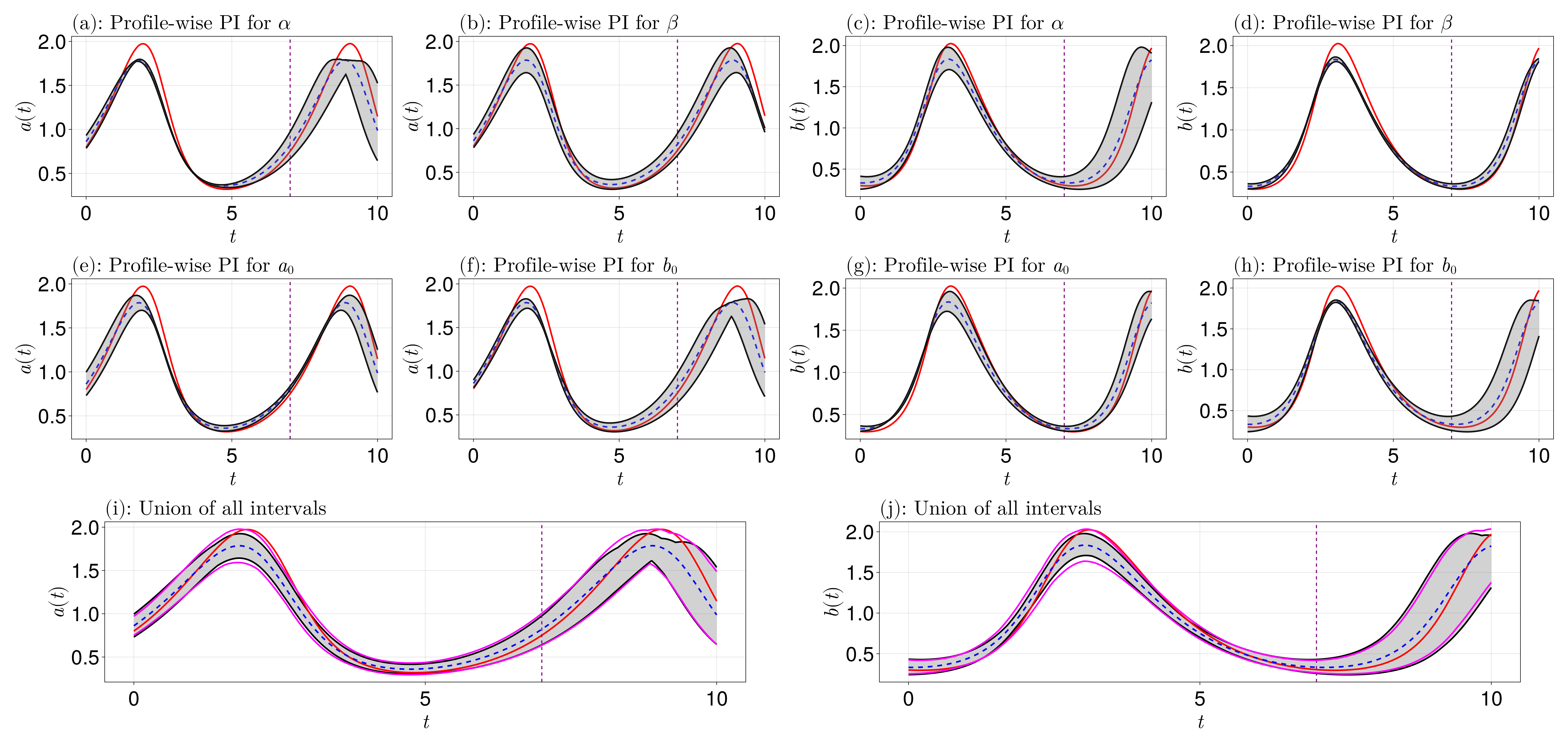

We see that the uncertainty around our predictions increases significantly for $t > 7$, as expected since we only use data in $0 \leq t \leq 7$ for estmiating the parameters. Moreover, the union intervals are good approximations to the intervals from the full likelihood.

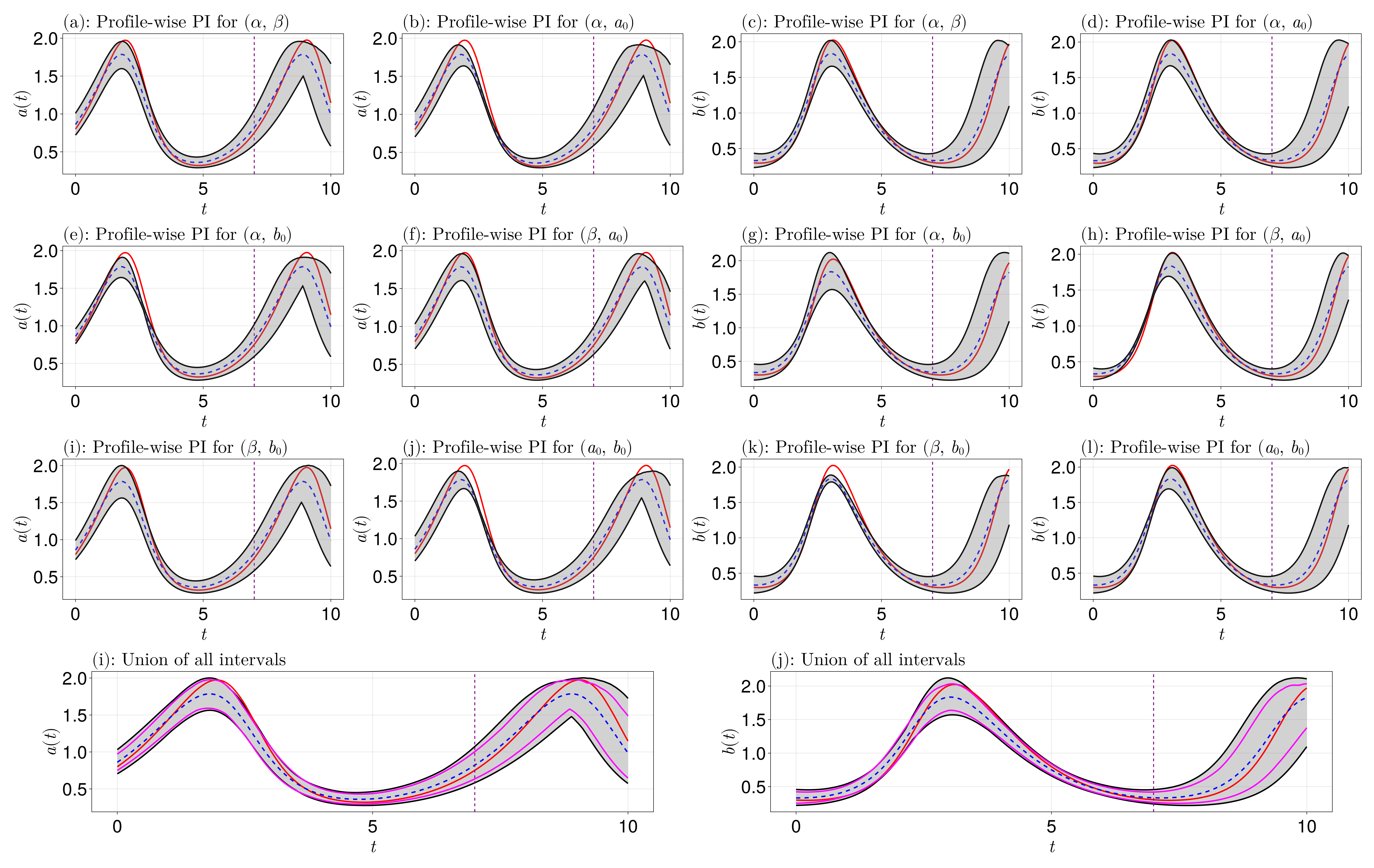
Now let us extend these results, instead computing prediction intervals from our bivariate profiles. The exact same function can be used for this.

# Bivariate prediction intervals 
individual_intervals, union_intervals, q_vals, param_ranges =
    get_prediction_intervals(prediction_function!, prof_2, pred_data; parallel=true,
        q_prototype)

# Plot the intervals 
fig = Figure(fontsize=38, size=(2935.488f0, 1854.64404f0))
integer_param_pairs = ProfileLikelihood.convert_symbol_tuples(param_pairs, prof_2) # converts to the integer representation
alp = [['a', 'b', 'e', 'f', 'i', 'j'], ['c', 'd', 'g', 'h', 'k', 'l']]
for (k, idx) in enumerate((a_idx, b_idx))
    for (i, (u, v)) in enumerate(integer_param_pairs)
        ax = Axis(fig[i < 3 ? 1 : (i < 5 ? 2 : 3), mod1(i, 2)+(k==2)*2], title=L"(%$(alp[k][i])): Profile-wise PI for (%$(latex_names[u]), %$(latex_names[v]))",
            titlealign=:left, width=600, height=300, xlabel=L"t", ylabel=k == 1 ? L"a(t)" : L"b(t)")
        vlines!(ax, [7.0], color=:purple, linestyle=:dash, linewidth=2)
        lines!(ax, t_many_pts, exact_soln[idx], color=:red, linewidth=3)
        lines!(ax, t_many_pts, mle_soln[idx], color=:blue, linestyle=:dash, linewidth=3)
        lines!(ax, t_many_pts, getindex.(individual_intervals[(u, v)], 1)[idx], color=:black, linewidth=3)
        lines!(ax, t_many_pts, getindex.(individual_intervals[(u, v)], 2)[idx], color=:black, linewidth=3)
        band!(ax, t_many_pts, getindex.(individual_intervals[(u, v)], 1)[idx], getindex.(individual_intervals[(u, v)], 2)[idx], color=(:grey, 0.35))
    end
end
a_ax = Axis(fig[4, 1:2], title=L"(i):$ $ Union of all intervals",
    titlealign=:left, width=1200, height=300, xlabel=L"t", ylabel=L"a(t)")
b_ax = Axis(fig[4, 3:4], title=L"(j):$ $ Union of all intervals",
    titlealign=:left, width=1200, height=300, xlabel=L"t", ylabel=L"b(t)")
_ax = (a_ax, b_ax)
for (k, idx) in enumerate((a_idx, b_idx))
    band!(_ax[k], t_many_pts, getindex.(union_intervals, 1)[idx], getindex.(union_intervals, 2)[idx], color=(:grey, 0.35))
    lines!(_ax[k], t_many_pts, getindex.(union_intervals, 1)[idx], color=:black, linewidth=3)
    lines!(_ax[k], t_many_pts, getindex.(union_intervals, 2)[idx], color=:black, linewidth=3)
    lines!(_ax[k], t_many_pts, exact_soln[idx], color=:red, linewidth=3)
    lines!(_ax[k], t_many_pts, mle_soln[idx], color=:blue, linestyle=:dash, linewidth=3)
    vlines!(_ax[k], [7.0], color=:purple, linestyle=:dash, linewidth=2)
end
for (k, idx) in enumerate((a_idx, b_idx))
    lines!(_ax[k], t_many_pts, q_lwr[idx], color=:magenta, linewidth=3)
    lines!(_ax[k], t_many_pts, q_upr[idx], color=:magenta, linewidth=3)
end