Example V: Moving boundary problem (Fisher-Stefan)
We now give an example where we perform profile likelihood analysis for a moving boundary problem, in particular the Fisher-Stefan problem (see e.g. this paper). This is a one-dimensional moving boundary problem. (If you want an example of a 2D PDE, you can see my paper here with associated package PoreBridging.jl – you can also see the docmuentation for ProfileLikelihood.jl for versions before 0.3.)
The packages we'll be using are loaded below.
using ProfileLikelihood
using MovingBoundaryProblems1D
using OrdinaryDiffEq
using LinearSolve
using Optimization
using CairoMakie
using OptimizationNLopt
using StableRNGs
The Fisher-Stefan problem is given by
\[\begin{array}{rcll} \dfrac{\partial u}{\partial t} & = & D\dfrac{\partial^2 u}{\partial x^2} + \lambda u\left(1-\dfrac{u}{K}\right) & 0 < x < L(t), \, t > 0,\\[9pt] \dfrac{\partial u}{\partial x} & = & 0 & x = 0,\,t>0, \\[9pt] u & = & 0 & x = L(t),\,t>0, \\[9pt] \dfrac{\mathrm dL}{\mathrm dt} & = & -\kappa\dfrac{\partial u}{\partial x} & x = L(t),\, t>0, \\[9pt] u(x, 0) & = & \begin{cases} \alpha & x < \beta, \\ 0 & x \geq \beta, \end{cases} & 0 \leq x \leq L(0), \\[9pt] L(0) &=& \beta, \end{array}\]
where $u$ is the population density, $D$ the diffusivity, $\lambda$ the proliferation rate, $K$ the carrying capacity density, and $\kappa$ is the Stefan parameter. The position of the leading edge is given by $L(t)$, initially given by $L(0)=\beta$. The parameters $(\lambda, K, D, \kappa)$ are what we are interested in estimating, letting $\alpha$ and $\beta$ be given by $1/2$ and $1$, respectively.
There are a few issues to consider when thinking about how to define a likelihood for this problem. Do we use define one based on individual values for $u(x_i, t_j)$? How do we compare solutions with different values of $L(t)$? Should we compare population densities and leading edges separately? The approach we take is to compare solutions by comparing the average density at each time. Namely, if we have times $t_1, \ldots, t_m$, and some solution $u(x, t)$, define the average density $M_i = M(t_i)$ to be
\[M_i = \dfrac{1}{L(t_i)}\int_0^{L(t_i)} u(x, t_i)\,\mathrm dx.\]
To evaluate this integral, let $\xi = x/L(t_i)$ so that $\mathrm d\xi = \mathrm dx/L(t_i)$, giving $M_i = \int_0^1 u(\xi, t_i)\,\mathrm d\xi$. We define our summary statistic using these average densities: Let the average density data be given by the time series $\{M_i^o\}_{i=1}^m$, and suppose for some parameter values $\boldsymbol \theta = (\lambda, K,D, \kappa)$ we compute densities $\{\hat M_i(\boldsymbol\theta)\}_{i=1}^m$. If we assume that the data $M_i^o$ are normally distributed around $\hat M_i(\boldsymbol \theta)$, meaning $M_i^o \sim \mathcal N(\hat M_i(\boldsymbol\theta), \sigma^2)$ for $i=1,\ldots,m$, then we have a Gaussian likelihood that we can use for estimation.
We need an extra component in our objective function. Just studying the average density will not be sufficient to get identifiable estimates for the parameters. Thus, we also take information about the position of the leading edge $L(t)$ over time. Similar arguments are used above for defining this leading edge as a normally distributed random variable. This ends up still leaving $\kappa$ unidentifiable, which we could assist by further improving the likelihood function, but we will not do that in this example.
We solve up to $t = 40$, but only use data at $t \leq 20$ for estimation.
Data generation
As usual, the first step in this problem is to generate the data. This requries us to first define the MBProblem and the method for evaluating $M_i$. (See the docs for MovingBoundaryProblems1D.jl for more information about setting up the MBProblem.)
## Define the problem
n = 100     # number of mesh points [making this a bit larger could give some better results, but it takes too long]
κ = [20.0]  # Stefan problem
α = 1 / 2   # initial condition height
β = 1.0     # initial endpoint
D = [0.89]  # diffusivity
λ = [1.1]   # proliferation rate
K = [3.0]   # carrying capacity density
T = 40.0    # final time
mesh_points = LinRange(0, β, n)
diffusion_function = (u, x, t, D) -> oftype(u, D[1])
reaction_function = (u, x, t, (λ, K)) -> λ[1] * u * (1 - u / K[1])
lhs = Neumann(0.0)
rhs = Dirichlet(0.0)
moving_boundary = Robin(
    (u, t, κ) -> (zero(u), oftype(u, -κ[1])),
    κ
)
ic = x -> x < β ? α : zero(x)
initial_condition = ic.(mesh_points)
prob = MBProblem(
    mesh_points, lhs, rhs, moving_boundary;
    diffusion_function,
    diffusion_parameters=D,
    reaction_function,
    reaction_parameters=(λ, K),
    initial_condition,
    initial_endpoint=β,
    final_time=T
)

## Generate the data
function compute_average(sol::AbstractVector, Δx)
    s = @views sol[begin:(end-1)]
    M = (s[1] + s[end]) / 2
    for i in 2:(length(s)-1)
        M += s[i]
    end
    M *= Δx
    return M
end
function compute_average(sol) # (1/L)∫₀ᴸ u(x, t) dx = ∫₀¹ u(ξ, t) dξ
    prob = sol.prob.p
    mesh_points = prob.geometry.mesh_points
    Δx = mesh_points[2] - mesh_points[1]
    M = map(sol) do _sol
        compute_average(_sol, Δx)
    end
    return M
end

sol = solve(prob, TRBDF2(linsolve=KLUFactorization()), saveat=T / 250)
M = compute_average(sol)
_original_M = deepcopy(M)
rng = StableRNG(123)
σM = 0.3
M .= max.(M .+ σM * randn(rng, length(M)), 0.0)
σL = 4.2
L = max.(sol[end, :] .+ σL * randn(rng, length(sol[end, :])), 0.0)
_original_L = deepcopy(sol[end, :])
With this setup, the data that we have is shown below.
fig = Figure(fontsize=41)
ax = Axis(fig[1, 1], width=1200, height=400,
    xlabel=L"t", ylabel=L"M(t)", titlealign=:left)
L1 = lines!(ax, sol.t, M, color=:black, linewidth=6)
L2 = lines!(ax, sol.t, _original_M, color=:red, linewidth=4)
axislegend(ax, [L1, L2], [L"$ $Noisy", L"$ $Original"], L"$ $Solution", position=:rb)
ax = Axis(fig[2, 1], width=1200, height=400,
    xlabel=L"t", ylabel=L"L(t)", titlealign=:left)
L1 = lines!(ax, sol.t, L, color=:black, linewidth=6)
L2 = lines!(ax, sol.t, _original_L, color=:red, linewidth=4)
axislegend(ax, [L1, L2], [L"$ $Noisy", L"$ $Original"], L"$ $Solution", position=:rb)
resize_to_layout!(fig)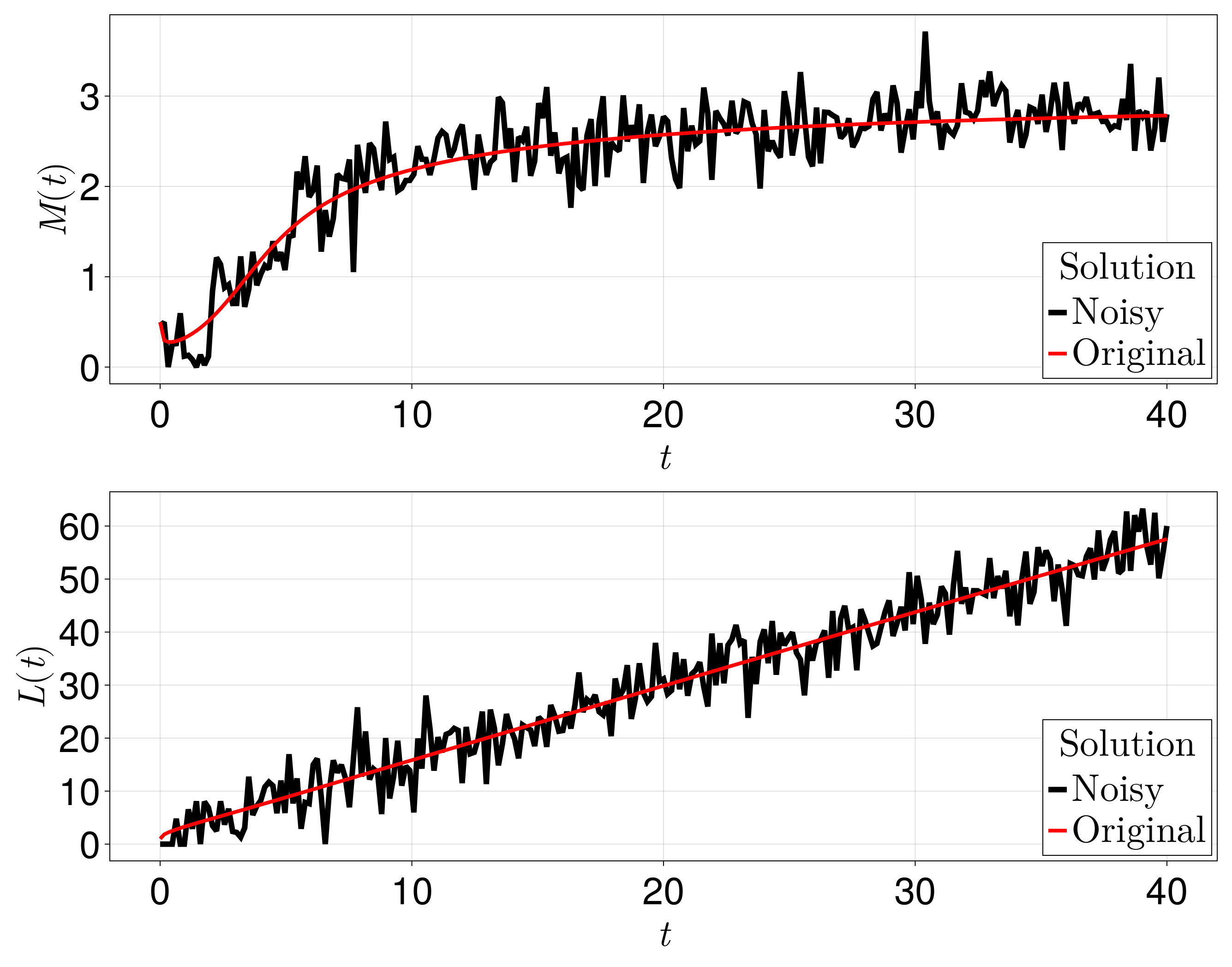
Defining the LikelihoodProblem
We now define our likelihood problem.
function mb_loglik(θ, data, integrator)
    λ, K, D, κ = θ
    M, L, n, σM, σL = data
    prob = integrator.p
    Δx = prob.geometry.mesh_points[2] - prob.geometry.mesh_points[1]
    prob.diffusion_parameters[1] = D
    prob.reaction_parameters[1][1] = λ
    prob.reaction_parameters[2][1] = K
    prob.boundary_conditions.moving_boundary.p[1] = κ
    reinit!(integrator)
    solve!(integrator)
    if !SciMLBase.successful_retcode(integrator.sol)
        return typemin(eltype(θ))
    end
    ℓ = zero(eltype(θ))
    for i in 1:n
        Mᵢ = compute_average(integrator.sol.u[i], Δx)
        ℓ = ℓ - 0.5log(2π * σM^2) - 0.5(M[i] - Mᵢ)^2 / σM^2
        Lᵢ = integrator.sol.u[i][end]
        ℓ = ℓ - 0.5log(2π * σL^2) - 0.5(L[i] - Lᵢ)^2 / σL^2
    end
    @show ℓ
    return ℓ
end
lb = [0.2, 0.5, 0.1, 10.0]
ub = [8.0, 8.0, 8.0, 40.0]
θ₀ = [0.5, 2.2, 0.5, 25.0]
syms = [:λ, :K, :D, :κ]
n = findlast(sol.t .≤ 20.0) # using t ≤ 20.0 for estimation
p = (M, L, n, σM, σL)
integrator = init(prob, TRBDF2(linsolve=KLUFactorization(; reuse_symbolic=false)); # https://github.com/JuliaSparse/KLU.jl/issues/12
    saveat=T / 250, verbose=false)
likprob = LikelihoodProblem(
    mb_loglik, θ₀, integrator;
    syms=syms,
    data=p,
    f_kwargs=(adtype=AutoFiniteDiff(),), # see https://github.com/SciML/Optimization.jl/issues/548
    prob_kwargs=(lb=lb, ub=ub))
Parameter estimation
Now let us do our parameter estimation.
@time mle_sol = mle(likprob, NLopt.LN_NELDERMEAD();
    xtol_abs=1e-4, xtol_rel=1e-4,
    ftol_abs=1e-4, ftol_rel=1e-4)
 96.699999 seconds (334.11 M allocations: 131.859 GiB, 7.00% gc time)
LikelihoodSolution. retcode: Success
Maximum likelihood: -383.6935496726186
Maximum likelihood estimates: 4-element Vector{Float64}
     λ: 1.1516248308036685
     K: 2.9884211752858167
     D: 1.1637069323254954
     κ: 11.443256674364815
@time prof = profile(likprob, mle_sol;
xtol_abs=1e-4, xtol_rel=1e-4,
ftol_abs=1e-4, ftol_rel=1e-4,
maxiters=100, maxtime=600,
parallel=true, resolution=60,
min_steps=20,
next_initial_estimate_method=:interp)
5087.412720 seconds (14.11 G allocations: 5.435 TiB, 4.59% gc time)
ProfileLikelihoodSolution. MLE retcode: Success
Confidence intervals:
95.0% CI for λ: (1.0308982572106475, 1.2575143923759817)
95.0% CI for K: (2.86631176866806, 3.1784886463924136)
95.0% CI for D: (0.6693749214281204, 1.4479573978872977)
95.0% CI for κ: (10.0, 40.0)fig = plot_profiles(prof;
latex_names=[L"\lambda", L"K", L"D", L"\kappa"],
show_mles=true,
shade_ci=true,
true_vals=[1.1, 3.0, 0.89, 20.0],
fig_kwargs=(fontsize=41,),
axis_kwargs=(width=600, height=300))
resize_to_layout!(fig)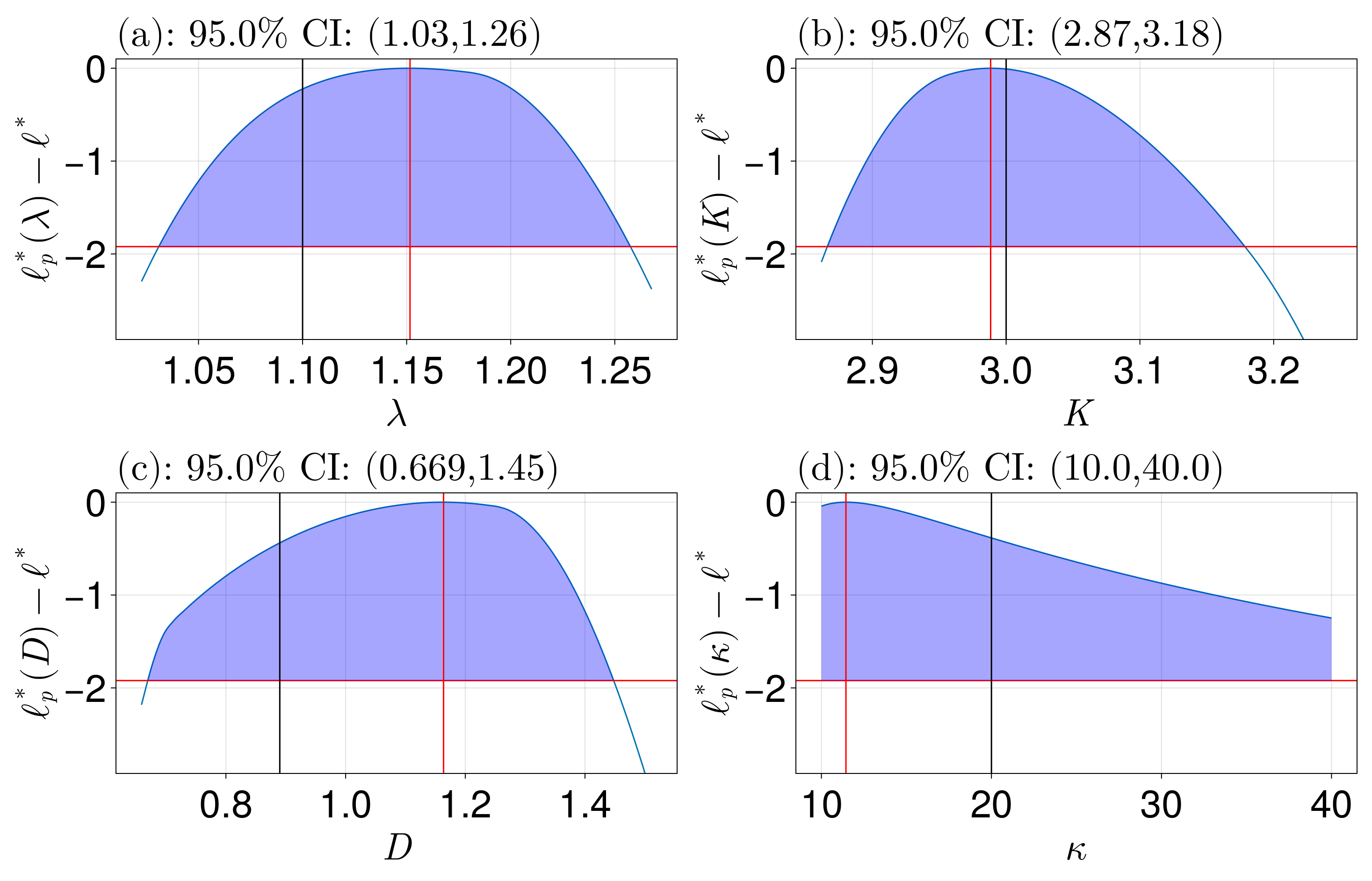
We see that all the parameters are well identified except for $\kappa$, which is perhaps not so surprising since the travelling waves that the solution evolves into are similar for $\kappa$ greater than some critical $\kappa=\kappa_c$.
Prediction intervals
Let's now compute some univariate prediction intervals. Note that we will be doing some extrapolation here, since we estimated with $0 \leq t \leq 20$ but we will predict up to $t = 40$. The quantity of interest here is $M(t)$.
function prediction_function!(q, θ::AbstractVector{T}, data) where {T}
    λ, K, D, κ = θ
    prob, t = data
    prob.diffusion_parameters[1] = D
    prob.reaction_parameters[1][1] = λ
    prob.reaction_parameters[2][1] = K
    prob.boundary_conditions.moving_boundary.p[1] = κ
    sol = solve(prob, TRBDF2(linsolve=KLUFactorization()), saveat=t)
    q .= compute_average(sol)
    return nothing
end
t_many_pts = LinRange(0, T, 1000)
pred_data = (prob, t_many_pts)
q_prototype = zero(t_many_pts)
individual_intervals, union_intervals, q_vals, param_ranges =
    get_prediction_intervals(prediction_function!, prof, pred_data; parallel=true,
        q_prototype)
Now let's plot these results, including the MLE and exact curves.
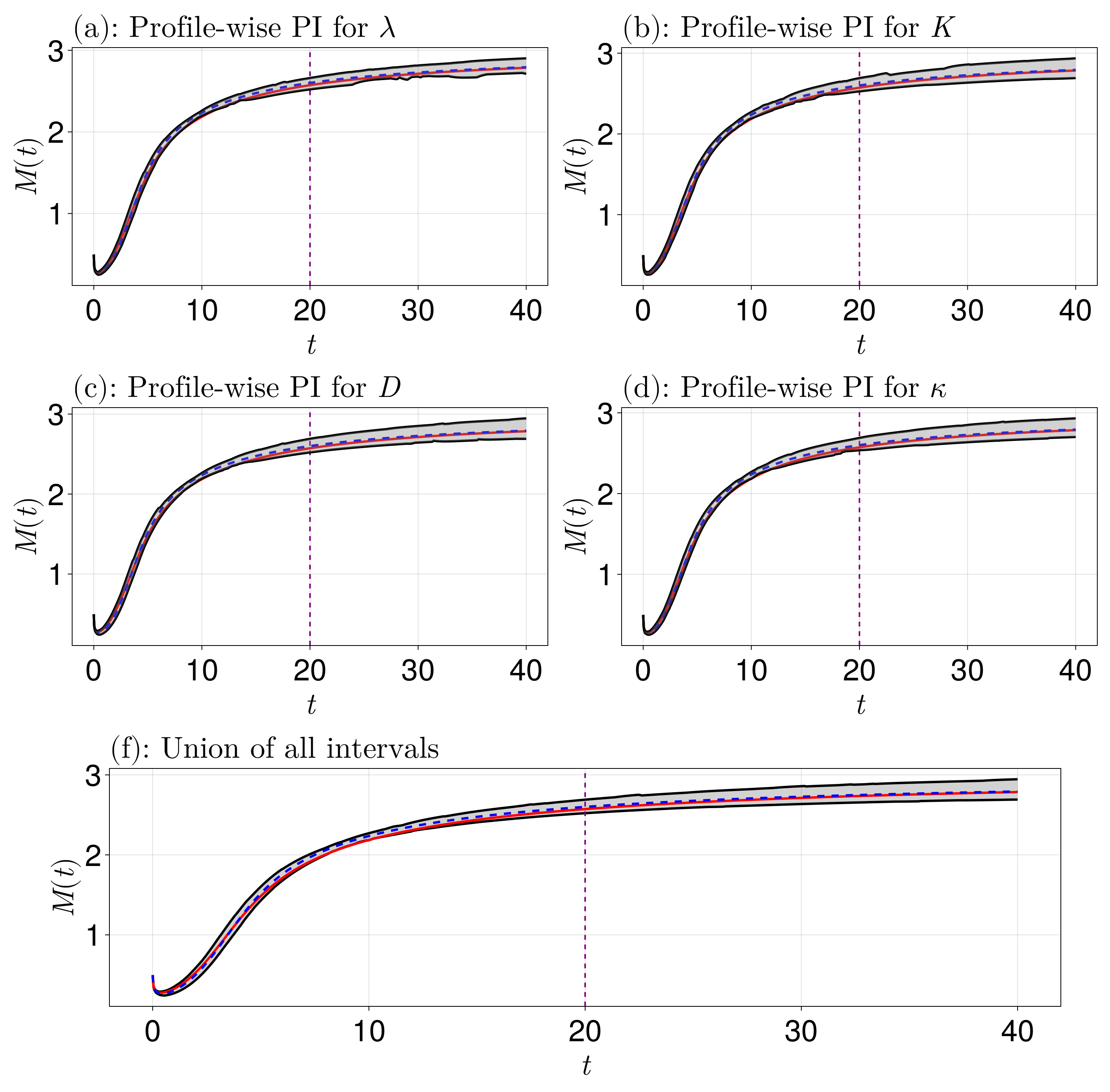
We see that the uncertainty covers the exact curves. We could keep going and doing e.g. bivariate profiles and bivariate prediction intervals, but let us stop here (see the Lotka-Volterra example in Example IV if you want to see bivariate profiling).