Comparison of Interpolation Methods
In this section, we will compare the methods available in this package for interpolation. We consider both quantitative and qualitative comparisons. We first make compares using errors around each point (local analysis), and later we compare errors using global metrics (global analysis). Note that there are many papers that compare interpolation methods, so if you really want a formal analysis that also considers other interpolation methods (like kriging or radial basis methods), you can search for them. The purpose here is to just show comparisons between the methods in this package, not to, say, argue that natural neighbour interpolation fits every possible situation, or to suggest that this is even the best way to perform such an analysis. You can find some good references in Bobach's thesis. A conclusion is given at the end of this section.
Setting up the Analysis
To setup this analysis, we use the following packages:
using NaturalNeighbours
using CairoMakie
using StableRNGs
using DelaunayTriangulation
using StaticArrays
using LinearAlgebra
using DataFrames
using StatsBase
using AlgebraOfGraphics
using BenchmarkTools
const NNI = NaturalNeighbours
We also define the following constants and other useful variables:
const itp_methods = (
    Sibson(0),
    Triangle(),
    Nearest(),
    Laplace(),
    Sibson(1),
    Farin(1),
    Hiyoshi(2)
)
const diff_methods = (
    Direct(),
    Iterative()
)
const itp_aliases = (:Sibson0, :Triangle, :Nearest, :Laplace, :Sibson1, :Farin, :Hiyoshi)
const diff_aliases = (:Direct, :Iterative)
const itp_alias_map = Dict(itp_methods .=> itp_aliases)
const diff_alias_map = Dict(diff_methods .=> diff_aliases)
const colors = Dict(itp_aliases .=> [:red, :blue, :green, :orange, :purple, :black, :brown])
const linestyles = Dict(diff_aliases .=> [:solid, :dashdotdot])
const line_elements = [
    LineElement(color=color,
        linewidth=22,
        linestyle=:solid) for color in values(colors)
]
const style_elements = [
    LineElement(color=:black,
        linewidth=22,
        linestyle=linestyle) for linestyle in values(linestyles)
]
const azimuths = [0.3, 0.8, 0.3, 0.6, 0.6, 0.6, 0.45]
rng = StableRNG(123)
xg = LinRange(0, 1, 25)
yg = LinRange(0, 1, 25)
x = vec([x for x in xg, _ in yg])
y = vec([y for _ in xg, y in yg])
xg2 = LinRange(0, 1, 250)
yg2 = LinRange(0, 1, 250)
xq = vec([x for x in xg2, _ in yg2])
yq = vec([y for _ in xg2, y in yg2])
tol = 1e-2
tri = triangulate([x'; y']; rng=rng)
triq = triangulate([xq'; yq']; rng=rng)
exterior_idx = identify_exterior_points(xq, yq, get_points(tri), get_convex_hull_vertices(tri); tol=tol)
interior_idx = filter(∉(exterior_idx), eachindex(xq, yq))
Lastly, we define the following test functions (the first six come from this report).
const f = [
    (x, y) -> 0.75 * exp(-((9 * x - 2)^2 + (9 * y - 2)^2) / 4) + 0.75 * exp(-(9 * x + 1)^2 / 49 - (9 * y + 1) / 10) + 0.5 * exp(-((9 * x - 7)^2 + (9 * y - 3)^2) / 4) - 0.2 * exp(-(9 * x - 4)^2 - (9 * y - 7)^2)
    (x, y) -> (1 / 9) * (tanh(9 * y - 9 * x) + 1)
    (x, y) -> (1.25 + cos(5.4 * y)) / (6 * (1 + (3 * x - 1)^2))
    (x, y) -> (1 / 3) * exp(-(81 / 16) * ((x - 1 / 2)^2 + (y - 1 / 2)^2))
    (x, y) -> (1 / 3) * exp(-(81 / 4) * ((x - 1 / 2)^2 + (y - 1 / 2)^2))
    (x, y) -> (1 / 9) * (64 - 81 * ((x - 1 / 2)^2 + (y - 1 / 2)^2))^(1 / 2) - 1 / 2
    (x, y) -> sin(27 * x * y) - exp(-(x - y)^2 / 4) * cos(13 * x - 13 * y)
]
const ∇f = [
    (x, y) -> @SVector[(exp(-(9 * x - 4)^2 - (9 * y - 7)^2) * (162 * x - 72)) / 5 - (3 * exp(-(9 * x - 2)^2 / 4 - (9 * y - 2)^2 / 4) * ((81 * x) / 2 - 9)) / 4 - (exp(-(9 * x - 7)^2 / 4 - (9 * y - 3)^2 / 4) * ((81 * x) / 2 - 63 / 2)) / 2 - (3 * exp(-(9 * y) / 10 - (9 * x + 1)^2 / 49 - 1 / 10) * ((162 * x) / 49 + 18 / 49)) / 4
        (exp(-(9 * x - 4)^2 - (9 * y - 7)^2) * (162 * y - 126)) / 5 - (3 * exp(-(9 * x - 2)^2 / 4 - (9 * y - 2)^2 / 4) * ((81 * y) / 2 - 9)) / 4 - (exp(-(9 * x - 7)^2 / 4 - (9 * y - 3)^2 / 4) * ((81 * y) / 2 - 27 / 2)) / 2 - (27 * exp(-(9 * y) / 10 - (9 * x + 1)^2 / 49 - 1 / 10)) / 40]
    (x, y) -> @SVector[tanh(9 * x - 9 * y)^2 - 1
        1 - tanh(9 * x - 9 * y)^2]
    (x, y) -> @SVector[-((108 * x - 36) * (cos((27 * y) / 5) + 5 / 4)) / (6 * (3 * x - 1)^2 + 6)^2
        -(27 * sin((27 * y) / 5)) / (5 * (6 * (3 * x - 1)^2 + 6))]
    (x, y) -> @SVector[-(exp(-(81 * (x - 1 / 2)^2) / 16 - (81 * (y - 1 / 2)^2) / 16) * ((81 * x) / 8 - 81 / 16)) / 3
        -(exp(-(81 * (x - 1 / 2)^2) / 16 - (81 * (y - 1 / 2)^2) / 16) * ((81 * y) / 8 - 81 / 16)) / 3]
    (x, y) -> @SVector[-(exp(-(81 * (x - 1 / 2)^2) / 4 - (81 * (y - 1 / 2)^2) / 4) * ((81 * x) / 2 - 81 / 4)) / 3
        -(exp(-(81 * (x - 1 / 2)^2) / 4 - (81 * (y - 1 / 2)^2) / 4) * ((81 * y) / 2 - 81 / 4)) / 3]
    (x, y) -> @SVector[-(162 * x - 81) / (18 * (64 - 81 * (y - 1 / 2)^2 - 81 * (x - 1 / 2)^2)^(1 / 2))
        -(162 * y - 81) / (18 * (64 - 81 * (y - 1 / 2)^2 - 81 * (x - 1 / 2)^2)^(1 / 2))]
    (x, y) -> @SVector[27 * y * cos(27 * x * y) + 13 * exp(-(x - y)^2 / 4) * sin(13 * x - 13 * y) + exp(-(x - y)^2 / 4) * cos(13 * x - 13 * y) * (x / 2 - y / 2)
        27 * x * cos(27 * x * y) - 13 * exp(-(x - y)^2 / 4) * sin(13 * x - 13 * y) - exp(-(x - y)^2 / 4) * cos(13 * x - 13 * y) * (x / 2 - y / 2)]
]
const Hf = [
    (x, y) -> @SMatrix[(162*exp(-(9 * x - 4)^2 - (9 * y - 7)^2))/5-(243*exp(-(9 * y) / 10 - (9 * x + 1)^2 / 49 - 1 / 10))/98-(243*exp(-(9 * x - 2)^2 / 4 - (9 * y - 2)^2 / 4))/8-(81*exp(-(9 * x - 7)^2 / 4 - (9 * y - 3)^2 / 4))/4+(3*exp(-(9 * y) / 10 - (9 * x + 1)^2 / 49 - 1 / 10)*((162*x)/49+18/49)^2)/4+(3*exp(-(9 * x - 2)^2 / 4 - (9 * y - 2)^2 / 4)*((81*x)/2-9)^2)/4+(exp(-(9 * x - 7)^2 / 4 - (9 * y - 3)^2 / 4)*((81*x)/2-63/2)^2)/2-(exp(-(9 * x - 4)^2 - (9 * y - 7)^2)*(162*x-72)^2)/5 (27*exp(-(9 * y) / 10 - (9 * x + 1)^2 / 49 - 1 / 10)*((162*x)/49+18/49))/40+(3*exp(-(9 * x - 2)^2 / 4 - (9 * y - 2)^2 / 4)*((81*x)/2-9)*((81*y)/2-9))/4+(exp(-(9 * x - 7)^2 / 4 - (9 * y - 3)^2 / 4)*((81*x)/2-63/2)*((81*y)/2-27/2))/2-(exp(-(9 * x - 4)^2 - (9 * y - 7)^2)*(162*x-72)*(162*y-126))/5
        (27*exp(-(9 * y) / 10 - (9 * x + 1)^2 / 49 - 1 / 10)*((162*x)/49+18/49))/40+(3*exp(-(9 * x - 2)^2 / 4 - (9 * y - 2)^2 / 4)*((81*x)/2-9)*((81*y)/2-9))/4+(exp(-(9 * x - 7)^2 / 4 - (9 * y - 3)^2 / 4)*((81*x)/2-63/2)*((81*y)/2-27/2))/2-(exp(-(9 * x - 4)^2 - (9 * y - 7)^2)*(162*x-72)*(162*y-126))/5 (243*exp(-(9 * y) / 10 - (9 * x + 1)^2 / 49 - 1 / 10))/400+(162*exp(-(9 * x - 4)^2 - (9 * y - 7)^2))/5-(243*exp(-(9 * x - 2)^2 / 4 - (9 * y - 2)^2 / 4))/8-(81*exp(-(9 * x - 7)^2 / 4 - (9 * y - 3)^2 / 4))/4+(3*exp(-(9 * x - 2)^2 / 4 - (9 * y - 2)^2 / 4)*((81*y)/2-9)^2)/4+(exp(-(9 * x - 7)^2 / 4 - (9 * y - 3)^2 / 4)*((81*y)/2-27/2)^2)/2-(exp(-(9 * x - 4)^2 - (9 * y - 7)^2)*(162*y-126)^2)/5]
    (x, y) -> @SMatrix[-2*tanh(9 * x - 9 * y)*(9*tanh(9 * x - 9 * y)^2-9) 2*tanh(9 * x - 9 * y)*(9*tanh(9 * x - 9 * y)^2-9)
        2*tanh(9 * x - 9 * y)*(9*tanh(9 * x - 9 * y)^2-9) -2*tanh(9 * x - 9 * y)*(9*tanh(9 * x - 9 * y)^2-9)]
    (x, y) -> @SMatrix[(2*(108*x-36)^2*(cos((27 * y) / 5)+5/4))/(6*(3*x-1)^2+6)^3-(108*(cos((27 * y) / 5)+5/4))/(6*(3*x-1)^2+6)^2 (27*sin((27 * y) / 5)*(108*x-36))/(5*(6*(3*x-1)^2+6)^2)
        (27*sin((27 * y) / 5)*(108*x-36))/(5*(6*(3*x-1)^2+6)^2) -(729 * cos((27 * y) / 5))/(25*(6*(3*x-1)^2+6))]
    (x, y) -> @SMatrix[(exp(-(81 * (x - 1 / 2)^2) / 16 - (81 * (y - 1 / 2)^2) / 16)*((81*x)/8-81/16)^2)/3-(27*exp(-(81 * (x - 1 / 2)^2) / 16 - (81 * (y - 1 / 2)^2) / 16))/8 (exp(-(81 * (x - 1 / 2)^2) / 16 - (81 * (y - 1 / 2)^2) / 16)*((81*x)/8-81/16)*((81*y)/8-81/16))/3
        (exp(-(81 * (x - 1 / 2)^2) / 16 - (81 * (y - 1 / 2)^2) / 16)*((81*x)/8-81/16)*((81*y)/8-81/16))/3 (exp(-(81 * (x - 1 / 2)^2) / 16 - (81 * (y - 1 / 2)^2) / 16)*((81*y)/8-81/16)^2)/3-(27*exp(-(81 * (x - 1 / 2)^2) / 16 - (81 * (y - 1 / 2)^2) / 16))/8]
    (x, y) -> @SMatrix[(exp(-(81 * (x - 1 / 2)^2) / 4 - (81 * (y - 1 / 2)^2) / 4)*((81*x)/2-81/4)^2)/3-(27*exp(-(81 * (x - 1 / 2)^2) / 4 - (81 * (y - 1 / 2)^2) / 4))/2 (exp(-(81 * (x - 1 / 2)^2) / 4 - (81 * (y - 1 / 2)^2) / 4)*((81*x)/2-81/4)*((81*y)/2-81/4))/3
        (exp(-(81 * (x - 1 / 2)^2) / 4 - (81 * (y - 1 / 2)^2) / 4)*((81*x)/2-81/4)*((81*y)/2-81/4))/3 (exp(-(81 * (x - 1 / 2)^2) / 4 - (81 * (y - 1 / 2)^2) / 4)*((81*y)/2-81/4)^2)/3-(27*exp(-(81 * (x - 1 / 2)^2) / 4 - (81 * (y - 1 / 2)^2) / 4))/2]
    (x, y) -> @SMatrix[-(162 * x - 81)^2/(36*(64-81*(y-1/2)^2-81*(x-1/2)^2)^(3/2))-9/(64-81*(y-1/2)^2-81*(x-1/2)^2)^(1/2) -((162 * x - 81) * (162 * y - 81))/(36*(64-81*(y-1/2)^2-81*(x-1/2)^2)^(3/2))
        -((162 * x - 81) * (162 * y - 81))/(36*(64-81*(y-1/2)^2-81*(x-1/2)^2)^(3/2)) -(162 * y - 81)^2/(36*(64-81*(y-1/2)^2-81*(x-1/2)^2)^(3/2))-9/(64-81*(y-1/2)^2-81*(x-1/2)^2)^(1/2)]
    (x, y) -> @SMatrix[(339*exp(-(x - y)^2 / 4)*cos(13 * x - 13 * y))/2-729*y^2*sin(27 * x * y)-exp(-(x - y)^2 / 4)*cos(13 * x - 13 * y)*(x/2-y/2)^2-26*exp(-(x - y)^2 / 4)*sin(13 * x - 13 * y)*(x/2-y/2) 27*cos(27 * x * y)-(339*exp(-(x - y)^2 / 4)*cos(13 * x - 13 * y))/2-729*x*y*sin(27 * x * y)+exp(-(x - y)^2 / 4)*cos(13 * x - 13 * y)*(x/2-y/2)^2+26*exp(-(x - y)^2 / 4)*sin(13 * x - 13 * y)*(x/2-y/2)
        27*cos(27 * x * y)-(339*exp(-(x - y)^2 / 4)*cos(13 * x - 13 * y))/2-729*x*y*sin(27 * x * y)+exp(-(x - y)^2 / 4)*cos(13 * x - 13 * y)*(x/2-y/2)^2+26*exp(-(x - y)^2 / 4)*sin(13 * x - 13 * y)*(x/2-y/2) (339*exp(-(x - y)^2 / 4)*cos(13 * x - 13 * y))/2-729*x^2*sin(27 * x * y)-exp(-(x - y)^2 / 4)*cos(13 * x - 13 * y)*(x/2-y/2)^2-26*exp(-(x - y)^2 / 4)*sin(13 * x - 13 * y)*(x/2-y/2)]
]
Assessment Metrics
We define here the methods we will use for assessing the quality of an interpolant.
Surface Smoothness
There are many ways to measure how rough or how smooth a surface is. I don't consider anything so complicated here, and instead I just compare normal vectors at each point. For a function $f$, the normal vector at a point $(x, y, f(x, y))$ is given by $(-\partial_xf, -\partial_yf, 1)/\sqrt{1 + \partial_xf^2 + \partial_yf^2}$.
For the interpolated surface, we cannot rely so readily on the generated gradients for this purpose. We instead triangulate the interpolated surface and then, for each point on the surface, take an angle-weighted average of the normal vectors at each triangle adjoining that point. The functions for computing this average are given below.
function normal_to_triangle(p₁, p₂, p₃, z₁, z₂, z₃)
    x₁, y₁ = getxy(p₁)
    x₂, y₂ = getxy(p₂)
    x₃, y₃ = getxy(p₃)
    Δ = x₁ * y₂ - x₂ * y₁ - x₁ * y₃ + x₃ * y₁ + x₂ * y₃ - x₃ * y₂
    s₁ = (y₂ - y₃) / Δ
    s₂ = (y₃ - y₁) / Δ
    s₃ = (y₁ - y₂) / Δ
    s₄ = (x₃ - x₂) / Δ
    s₅ = (x₁ - x₃) / Δ
    s₆ = (x₂ - x₁) / Δ
    α = s₁ * z₁ + s₂ * z₂ + s₃ * z₃
    β = s₄ * z₁ + s₅ * z₂ + s₆ * z₃
    ∇norm = sqrt(1 + α^2 + β^2)
    ∇ = @SVector[-α, -β, 1.0]
    return ∇ / ∇norm
end
function normal_to_triangle(tri, z, i, j, k)
    p₁, p₂, p₃ = get_point(tri, i, j, k)
    z₁, z₂, z₃ = z[i], z[j], z[k]
    return normal_to_triangle(p₁, p₂, p₃, z₁, z₂, z₃)
end

function ∠(v₁, v₂)
    # acos is not reliable: https://people.eecs.berkeley.edu/~wkahan/Triangle.pdf, https://scicomp.stackexchange.com/a/27694/42528
    a = norm(v₁)
    b = norm(v₂)
    c = norm(v₁ - v₂)
    if a < b
        a, b = b, a
    end
    μ = if b ≥ c
        c - (a - b)
    else
        b - (a - c)
    end
    num = ((a - b) + c) * μ
    den = (a + (b + c)) * ((a - c) + b)
    θ = 2atan(sqrt(num / den))
    return θ
end
function ∠(tri, z, i, j, k)
    # Angle between pᵢpⱼ and pᵢpₖ
    p₁, p₂, p₃ = get_point(tri, i, j, k)
    z₁, z₂, z₃ = z[i], z[j], z[k]
    px, py = getxy(p₁)
    qx, qy = getxy(p₂)
    rx, ry = getxy(p₃)
    v₁ = @SVector[qx - px, qy - py, z₂ - z₁]
    v₂ = @SVector[rx - px, ry - py, z₃ - z₁]
    return ∠(v₁, v₂)
end

function average_normal_vector(tri, z, i)
    # Using the mean-weighted-angle formula: https://doi.org/10.1007/s00371-004-0271-1
    n = @SVector[0.0, 0.0, 1.0]
    neighbouring_edges = get_adjacent2vertex(tri, i)
    for (j, k) in neighbouring_edges
        if !DelaunayTriangulation.is_ghost_triangle(i, j, k)
            ψ = ∠(tri, z, i, j, k)
            n = n + ψ * normal_to_triangle(tri, z, i, j, k)
        end
    end
    return n / norm(n)
end

function compare_normal_vectors(tri, z, i, ∇f::Function)
    # Maybe this is similar to https://doi.org/10.1007/978-3-319-40548-3_19?
    # The description is so vague.
    p = get_point(tri, i)
    x, y = getxy(p)
    n̄̂ = average_normal_vector(tri, z, i)
    nx, ny = ∇f(x, y)
    n = @SVector[-nx, -ny, 1.0]
    n̂ = n / norm(n)
    return rad2deg(∠(n̄̂, n̂))
end
function compare_normal_vectors(tri, z, ∇f::Function, interior_idx)
    return [compare_normal_vectors(tri, z, i, ∇f) for i in interior_idx]
end
Comparing Raw Values Locally
To compare raw values, such as heights or Hessians, we use the error definition $\varepsilon(y, y\hat) = 2\|y - y\hat\| / \|y + y\hat\|$:
function compare_quantities(ŷ, y, interior_idx)
    ε = 2norm.(ŷ .- y) ./ norm.(ŷ .+ y)
    return to_unit(ε[interior_idx])
end
function to_unit(μ)
    return max.(μ, sqrt(eps(Float64)))
end
to_mat(H) = @SMatrix[H[1] H[3]; H[3] H[2]]
Local Analysis Function
The function we use for our local analysis is defined below.
function analysis_function!(df, tri, triq, x, y, xq, yq, fidx, itp_method, diff_method, interior_idx)
    g = f[fidx]
    ∇g = ∇f[fidx]
    Hg = Hf[fidx]
    z = g.(x, y)
    itp = interpolate(tri, z; derivatives=true, method=diff_method)
    ∂ = differentiate(itp, 2)

    ẑ = itp(xq, yq; method=itp_method)
    ∇̂Ĥ = ∂(xq, yq; method=diff_method, interpolant_method=itp_method)
    ∇̂ = SVector{2,Float64}.(first.(∇̂Ĥ))
    Ĥ = to_mat.(last.(∇̂Ĥ))

    z = g.(xq, yq)
    ∇ = ∇g.(xq, yq)
    H = Hg.(xq, yq)
    εz = compare_quantities(ẑ, z, interior_idx)
    ε∇ = compare_quantities(∇̂, ∇, interior_idx)
    εH = compare_quantities(Ĥ, H, interior_idx)
    εn = compare_normal_vectors(triq, ẑ, ∇g, interior_idx)

    _df = DataFrame(
        :z_exact => z[interior_idx],
        :z_approx => ẑ[interior_idx],
        :∇_exact => ∇[interior_idx],
        :∇_approx => ∇̂[interior_idx],
        :H_exact => H[interior_idx],
        :H_approx => Ĥ[interior_idx],
        :z_error => εz,
        :∇_error => ε∇,
        :H_error => εH,
        :n_error => εn,
        :itp_method => itp_alias_map[itp_method],
        :diff_method => diff_alias_map[diff_method],
        :f_idx => fidx
    )
    append!(df, _df)
    return df
end
function analysis_function(tri, triq, x, y, xq, yq, interior_idx)
    df = DataFrame(
        z_exact=Float64[],
        z_approx=Float64[],
        ∇_exact=SVector{2,Float64}[],
        ∇_approx=SVector{2,Float64}[],
        H_exact=SMatrix{2, 2, Float64}[],
        H_approx=SMatrix{2, 2, Float64}[],
        z_error=Float64[],
        ∇_error=Float64[],
        H_error=Float64[],
        n_error=Float64[],
        itp_method=Symbol[],
        diff_method=Symbol[],
        f_idx=Int[]
    )
    for fidx in eachindex(f, ∇f, Hf)
        for itp_method in itp_methods
            for diff_method in diff_methods
                analysis_function!(df, tri, triq, x, y, xq, yq, fidx, itp_method, diff_method, interior_idx)
            end
        end
    end
    return df
end
Quantitative Local Analysis
Let's now give the results for our quantitative local analysis. We use our analysis_function as:
df = analysis_function(tri, triq, x, y, xq, yq, interior_idx)
gdf = groupby(df, [:f_idx, :itp_method, :diff_method])
We plot these results as follows.
const alph = join('a':'z')
fig = Figure(fontsize=64)
z_ax = [Axis(fig[i, 1], xlabel=L"\varepsilon", ylabel=L"F(\varepsilon)",
    title=L"(%$(alph[i])1): $z$ $\varepsilon$ for $f_{%$i}", titlealign=:left,
    width=600, height=400, xscale=log10) for i in eachindex(f, ∇f, Hf)]
∇_ax = [Axis(fig[i, 2], xlabel=L"\varepsilon", ylabel=L"F(\varepsilon)",
    title=L"(%$(alph[i])2): $\nabla$ $\varepsilon$ for $f_{%$i}", titlealign=:left,
    width=600, height=400, xscale=log10) for i in eachindex(f, ∇f, Hf)]
H_ax = [Axis(fig[i, 3], xlabel=L"\varepsilon", ylabel=L"F(\varepsilon)",
    title=L"(%$(alph[i])3): $H$ $\varepsilon$ for $f_{%$i}", titlealign=:left,
    width=600, height=400, xscale=log10) for i in eachindex(f, ∇f, Hf)]
n_ax = [Axis(fig[i, 4], xlabel=L"\varepsilon", ylabel=L"F(\varepsilon)",
    title=L"(%$(alph[i])4): $n$ $\varepsilon$ for $f_{%$i}", titlealign=:left,
    width=600, height=400) for i in eachindex(f, ∇f, Hf)]
f_ax = [Axis3(fig[i, 5], xlabel=L"x", ylabel=L"y", zlabel=L"f_{%$i}(x, y)",
    title=L"(%$(alph[i])5): $f_{%$i}$'s surface", titlealign=:left,
    width=600, height=400, azimuth=azimuths[i]) for i in eachindex(f, ∇f, Hf)]
xℓ = [
    (1e-5, 1.0) (1e-3, 1.0) (1e-2, 1.0) (0.0, 5.0)
    (1e-5, 1.0) (1e-2, 1.0) (1e-1, 1.0) (0.0, 5.0)
    (1e-6, 1e-1) (1e-5, 1.0) (1e-2, 1.0) (0.0, 2.0)
    (1e-6, 1e-1) (1e-4, 1e-1) (1e-2, 1.0) (0.0, 1.0)
    (1e-5, 1e-1) (1e-3, 1.0) (1e-2, 1.0) (0.0, 2.0)
    (1e-8, 1e-1) (1e-5, 1e-1) (1e-2, 1e-1) (0.0, 0.5)
    (1e-2, 1.0) (1e-2, 1.0) (1e-1, 1.0) (0.0, 15.0)
]
for i in eachindex(f)
    xlims!(z_ax[i], xℓ[i, 1]...)
    xlims!(∇_ax[i], xℓ[i, 2]...)
    xlims!(H_ax[i], xℓ[i, 3]...)
    xlims!(n_ax[i], xℓ[i, 4]...)
end
for (f_idx, itp_alias, diff_alias) in keys(gdf)
    _df = gdf[(f_idx, itp_alias, diff_alias)]
    clr = colors[itp_alias]
    ls = linestyles[diff_alias]
    _z_ax = z_ax[f_idx]
    _∇_ax = ∇_ax[f_idx]
    _H_ax = H_ax[f_idx]
    _n_ax = n_ax[f_idx]
    z_error = _df.z_error
    ∇_error = _df.∇_error
    H_error = _df.H_error
    n_error = _df.n_error
    ecdfplot!(_z_ax, z_error, color=clr, linestyle=ls, linewidth=7)
    ecdfplot!(_∇_ax, ∇_error, color=clr, linestyle=ls, linewidth=7)
    ecdfplot!(_H_ax, H_error, color=clr, linestyle=ls, linewidth=7)
    if itp_alias ≠ :Nearest
        ecdfplot!(_n_ax, n_error, color=clr, linestyle=ls, linewidth=7)
    end
end
for f_idx in eachindex(f)
    g = f[f_idx]
    fz = [g(x, y) for x in xg2, y in yg2]
    _f_ax = f_ax[f_idx]
    surface!(_f_ax, xg2, yg2, fz)
end
[Legend(
    fig[i:(i+1), 6],
    [line_elements, style_elements],
    [string.(keys(colors)), string.(keys(linestyles))],
    ["Interpolant", "Differentiator"],
    titlesize=78,
    labelsize=78,
    patchsize=(100, 30)
) for i in (1, 3, 5)]
resize_to_layout!(fig)
fig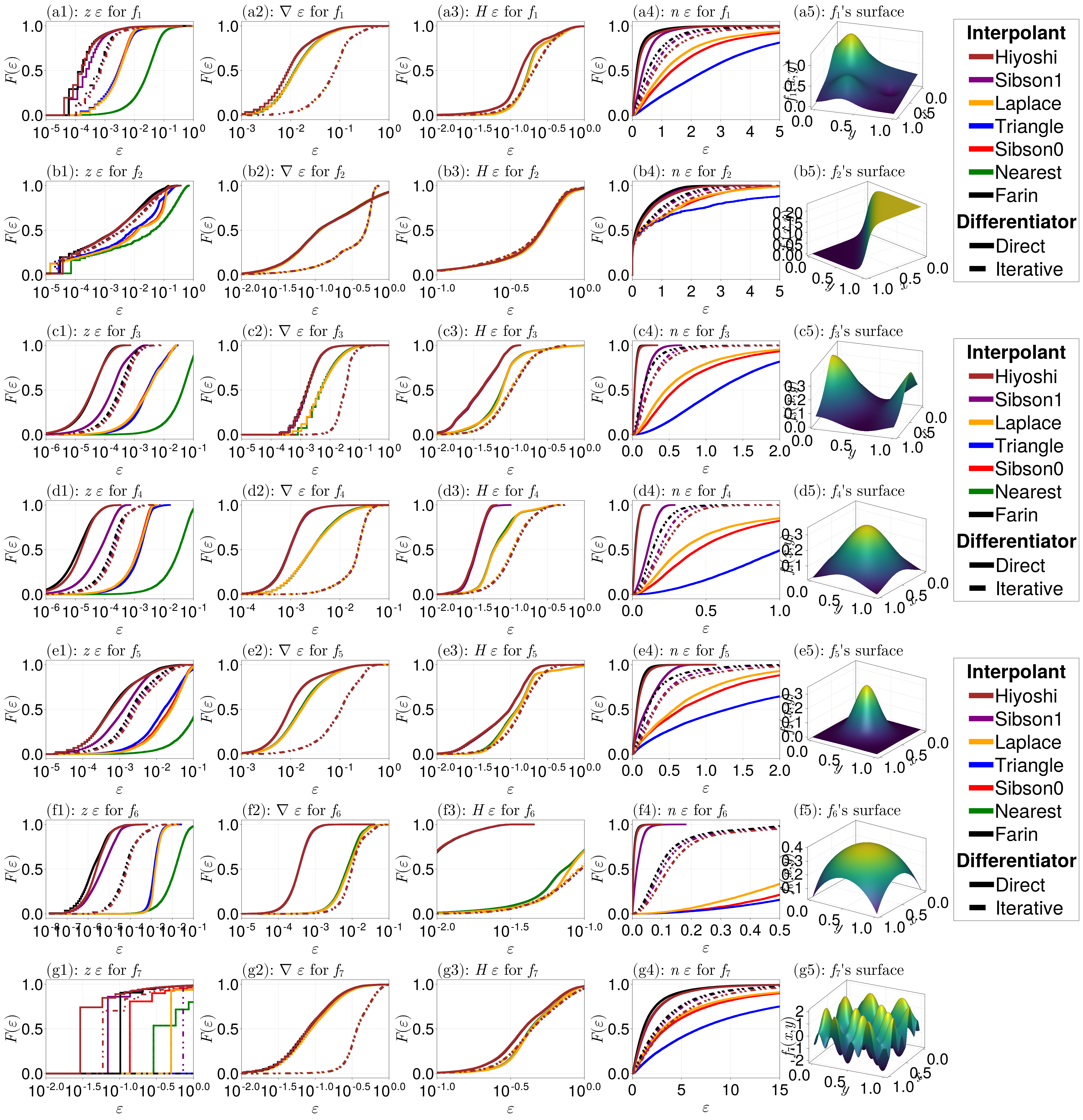
For these plots:
- The first column shows the errors for the height values.
- The second column shows the errors in the gradients.
- The third column shows the errors in the Hessians.
- The fourth column shows the errors in the normal vectors. The nearest neighbour interpolant is not shown for this column since it is (unsurprisingly) consistently the worst method.
- The fifth column shows the exact surface.
Note that we use the empirical cumulative distribution function, and the function $F(\varepsilon)$ in the $y$-axis could also be interpreted as the ``fraction of data''. For example, the plot in (f3) shows the curve for the Hiyoshi interpolant being much further to the left than the other curves, implying that Hiyoshi has by far outperformed the others.
Let us discuss what we see from each column.
The smooth interpolants (
Sibson(1),Farin(1), andHiyoshi(2)) seem to have the best performance here, with derivative information generated with the direct method, appear to perform the best when measuring differences in heights, with the nearest neighbour interpolant having the worst performance. TheLaplace(),Triangle(), andSibson(0)interpolants seem to have similar performance, although theTriangle()interpolant probably wouldn't have as high a performance if we had e.g. randomly spaced data (analysed later).The gradient estimates seem to depend only on the smoothness of the interpolant rather than the interpolant itself, and the
Direct()method seems to outperform theIterative()method for generating derivatives. In particular, for generating gradients, theHiyoshi(2),Sibson(1), orFarin(1)interpolants perform equally as well, provided theDirect()method is used.The results for the Hessians are similar to the gradient results.
For the smoothness of the interpolated surfaces, the
Hiyoshi(2)andFarin(1)results are consistently the best, withSibson(1)a close competitor. TheTriangle()interpolant leads to the least smooth surface of those considered. Similarly to the gradient and Hessians results, theDirect()approach leads to the best results compared toIterative().
Overall, the smooth interpolants lead to the best results, and of the non-smooth interpolants (Sibson(0), Laplace(), Triangle(), Nearest()), Sibson(0) seems to have the best results. For derivative generation, Direct() seems to give the best results.
Note that the analysis here does not consider whether using cubic terms in Direct() methods makes a difference, or whether varying alpha for the Iterative() approach makes a difference.
Qualitative Local Analysis
Now we will visualise the surfaces produced by the interpolants. Based on the above results, we will only consider Direct() for derivative generation. Let us first look at the surfaces themselves.
considered_itp = eachindex(itp_methods)
considered_fidx = eachindex(f)
fig = Figure(fontsize=72, resolution = (4800, 4900))
ax = [
    Axis3(fig[i, j],
        xlabel=L"x",
        ylabel=L"y",
        zlabel=L"f(x, y)",
        title=L"(%$(alph[i])%$(j)): ($f_{%$i}$, %$(itp_aliases[j]))",
        titlealign=:left,
        width=600,
        height=600,
        azimuth=azimuths[i]
    )
    for i in considered_fidx, j in considered_itp
]
for (j, i) in enumerate(considered_fidx)
    for (ℓ, k) in enumerate(considered_itp)
        _gdf = gdf[(i, itp_aliases[k], diff_aliases[1])]
        _ax = ax[j, ℓ]
        _z = _gdf.z_approx
        surface!(_ax, xq[interior_idx], yq[interior_idx], _z)
        xlims!(_ax, 0, 1)
        ylims!(_ax, 0, 1)
        hidedecorations!(_ax)
    end
end
fig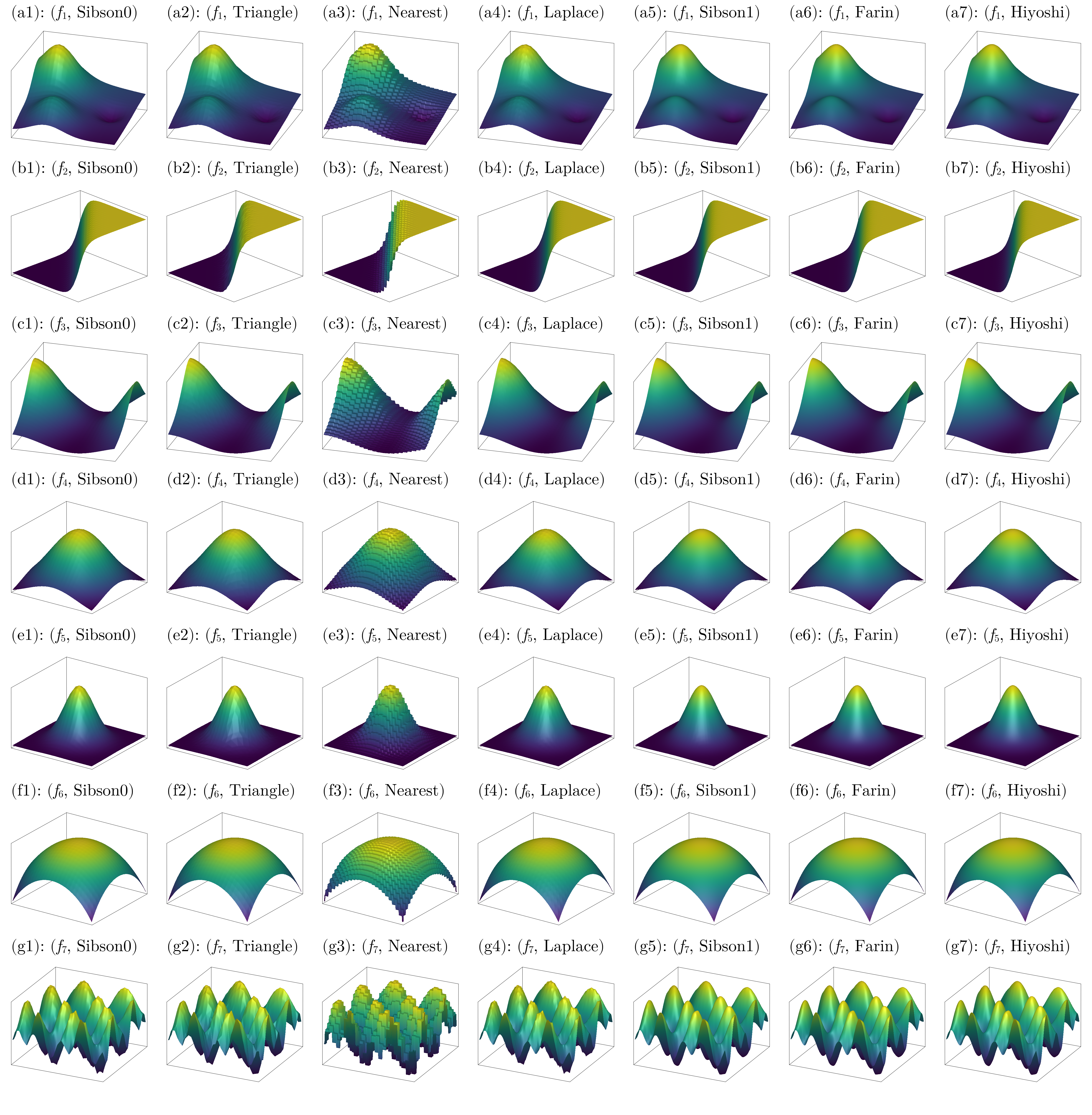
We can clearly see some of the roughness produced by the non-smooth interpolants. Hiyoshi(2) seems to have the best visual quality.
To assess these results further, we can look at the errors. The function we use for this is:
function plot_errors(considered_fidx, considered_itp, gdf, interior_idx, error_type, colorranges)
    fig = Figure(fontsize=72)
    ax = [
        Axis(fig[i, j],
            xlabel=L"x",
            ylabel=L"y",
            title=L"(%$(alph[i])%$(j)): ($f_{%$i}$, %$(itp_aliases[j]))",
            titlealign=:left,
            width=600,
            height=600,
        )
        for i in considered_fidx, j in considered_itp
    ]
    for (j, i) in enumerate(considered_fidx)
        for (ℓ, k) in enumerate(considered_itp)
            _gdf = gdf[(i, itp_aliases[k], diff_aliases[1])]
            _ax = ax[j, ℓ]
            ε = _gdf[!, error_type]
            heatmap!(_ax, xq[interior_idx], yq[interior_idx], ε, colorrange=colorranges[j])
            xlims!(_ax, 0, 1)
            ylims!(_ax, 0, 1)
            hidedecorations!(_ax)
        end
    end
    resize_to_layout!(fig)
    fig
end
For the height errors:
z_colorranges = [(1e-4, 0.01), (1e-5, 0.1), (1e-3, 0.05), (1e-4, 0.01), (1e-3, 0.1), (1e-4, 0.01), (1e-2, 0.5)]
fig = plot_errors(considered_fidx, considered_itp, gdf, interior_idx, :z_error, z_colorranges)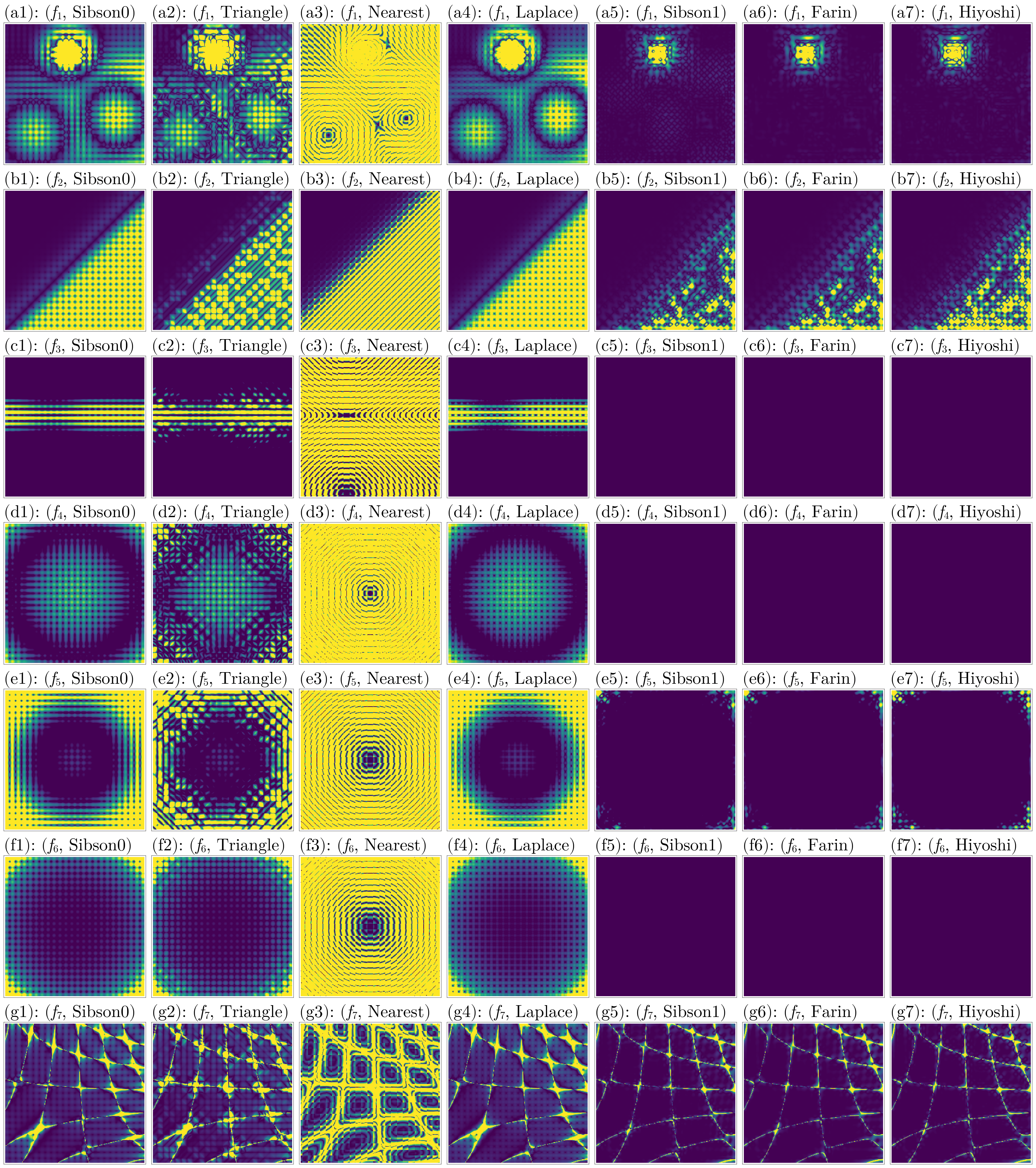
To compare the gradients, we use:
∇_colorranges = [(1e-2, 0.2), (1e-2, 1.0), (1e-2, 0.01), (1e-3, 0.01), (1e-2, 0.05), (1e-3, 0.01), (1e-2, 0.25)]
fig = plot_errors(considered_fidx, considered_itp, gdf, interior_idx, :∇_error, ∇_colorranges)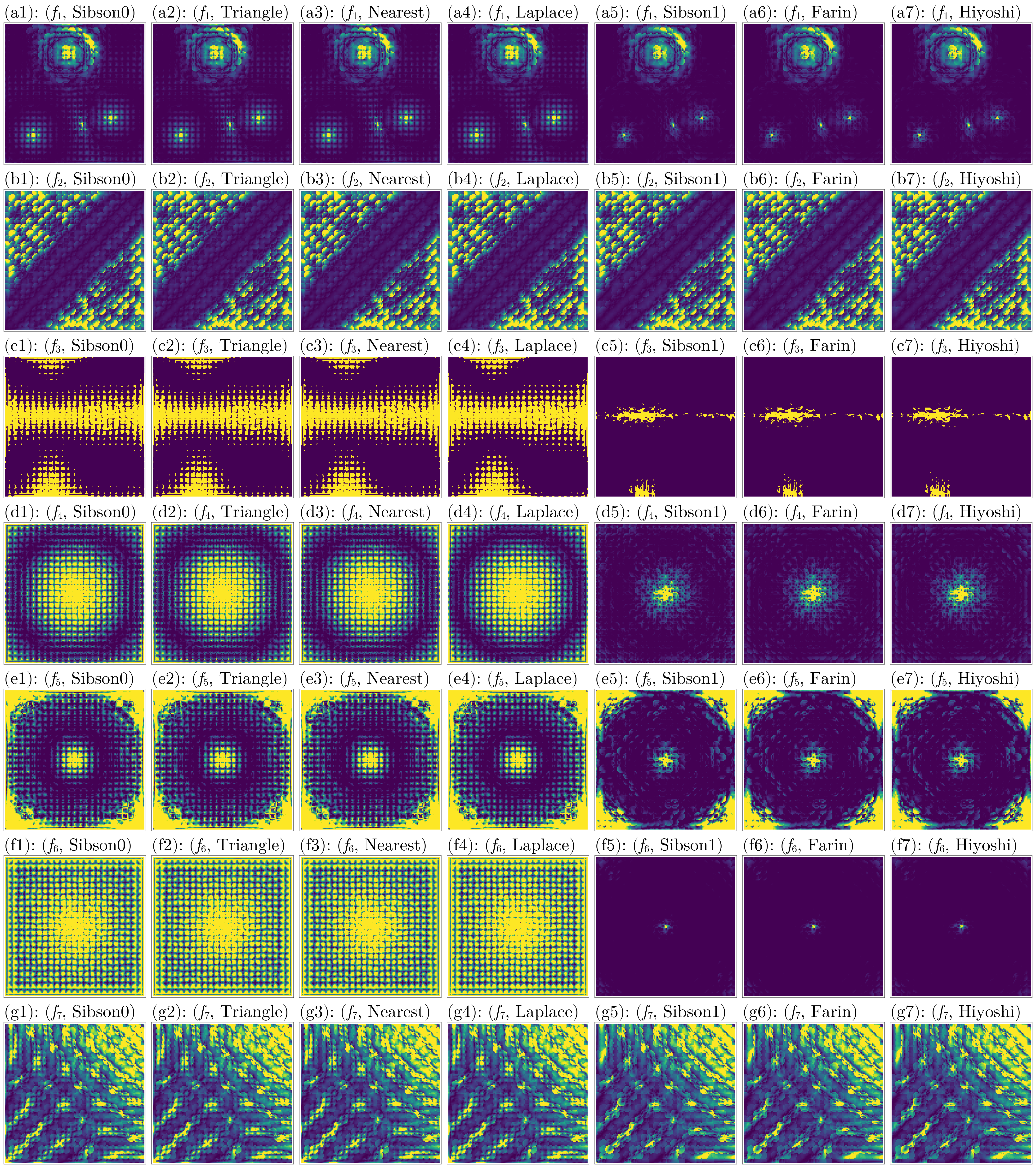
Next, the Hessians are compared:
H_colorranges = [(1e-1, 0.5), (0.2, 0.8), (1e-1, 0.2), (1e-2, 0.2), (1e-1, 0.25), (1e-2, 0.1), (1e-1, 0.8)]
fig = plot_errors(considered_fidx, considered_itp, gdf, interior_idx, :H_error, H_colorranges)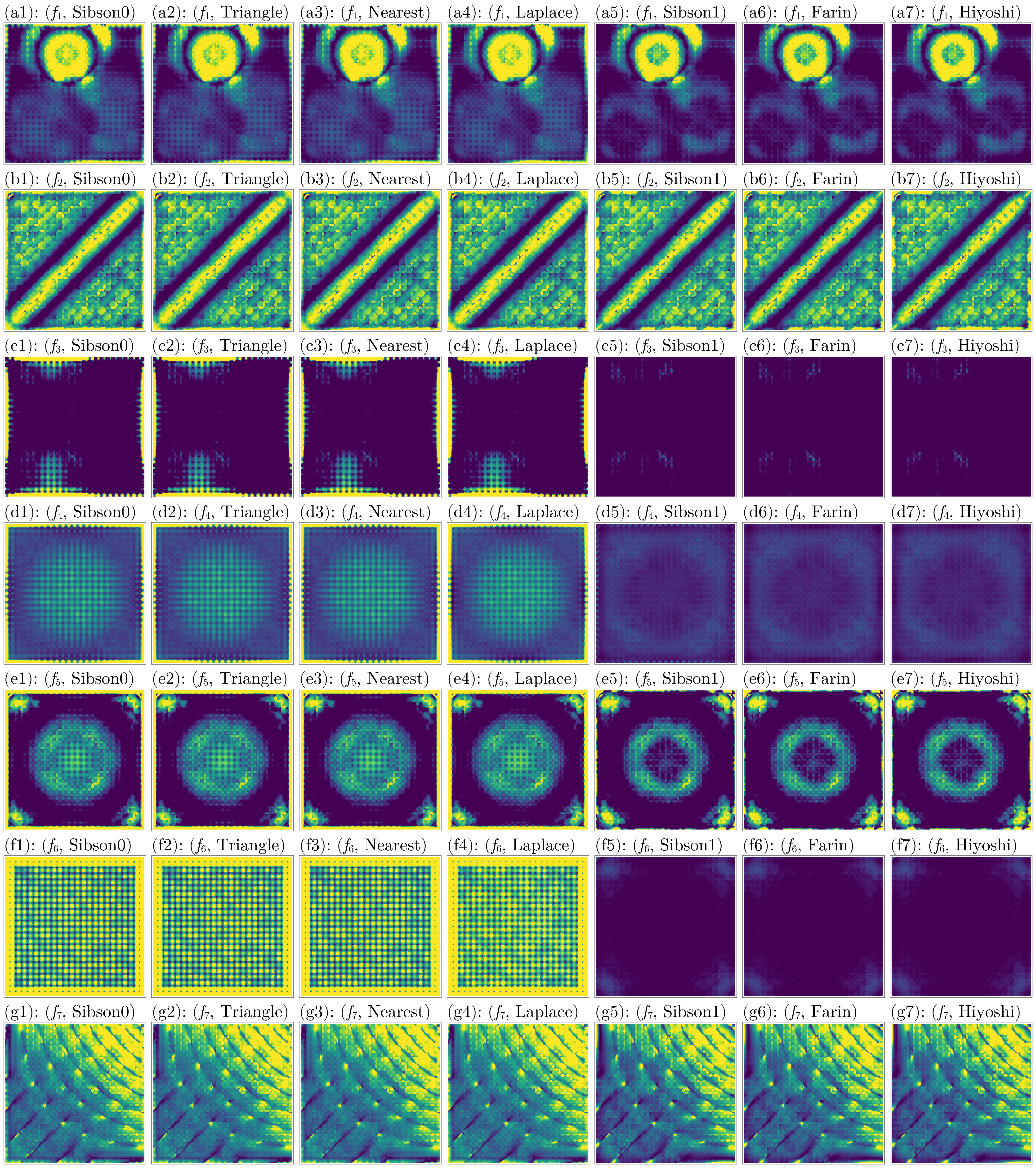
Finally, we compare the normal vector fields:
n_colorranges = [(0, 5), (0, 5), (0, 2), (0, 1), (0, 2), (0, 2.5), (0, 15)]
fig = plot_errors(considered_fidx, considered_itp, gdf, interior_idx, :n_error, n_colorranges)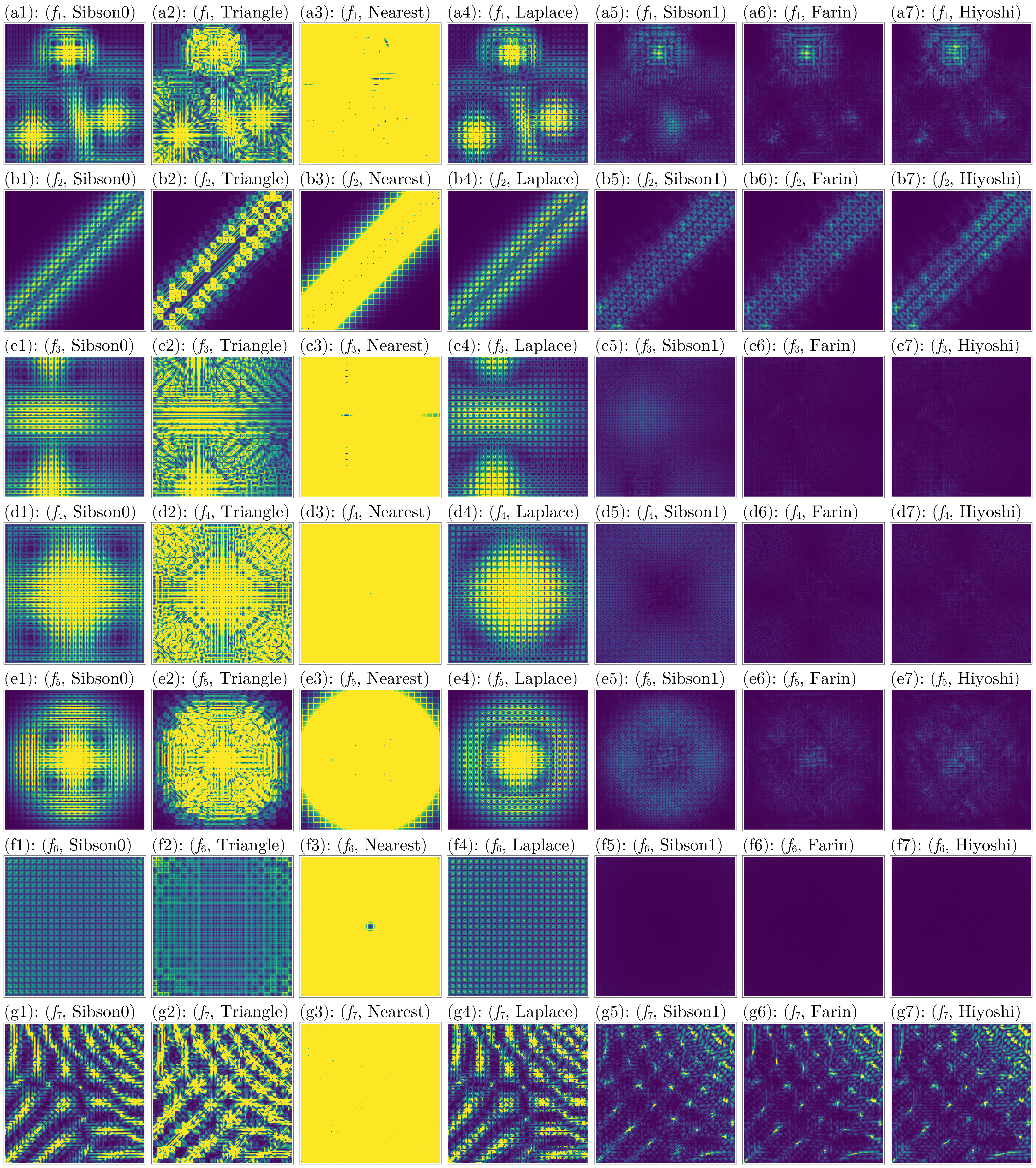
Judging from these results, again the Hiyoshi(2) and Farin(1) methods have the best performance across all metrics.
Quantitative Global Analysis
Now we will use global metrics to assess the interpolation quality. A limitation of the above discussion is that we are considering a fixed data set. Here, we instead consider random data sets (with the same test functions) and weighted averages of the local errors. We will measure the errors as a function of the median edge length of the data set's underlying triangulation. Note that, in these random data sets, we will not maintain a convex hull of $[0, 1]^2$. Lastly, we will use a stricter tolerance on whether to classify a point as being inside of the convex hull in this case, now using a tol = 0.1 rather than tol = 0.01. The global metric we use is $100\sqrt{\frac{\sum_i \|y_i - \hat y_i\|^2}{\sum_j \|\hat y_i\|^2}}$:
function rrmse(y, ŷ) # interior_indices already applied
    num = 0.0
    den = 0.0
    for (yᵢ, ŷᵢ) in zip(y, ŷ)
        if all(isfinite, (yᵢ..., ŷᵢ...))
            num += norm(yᵢ .- ŷᵢ)^2
            den += norm(ŷᵢ)^2
        end
    end
    return 100sqrt(num / den)
end
For comparing the normal vector errors, we will just use the median. To compute the median edge length of a triangulation, we use:
function median_edge_length(tri)
    lengths = zeros(DelaunayTriangulation.num_solid_edges(tri))
    for (k, (i, j)) in (enumerate ∘ each_solid_edge)(tri)
        p, q = get_point(tri, i, j)
        px, py = getxy(p)
        qx, qy = getxy(q)
        ℓ = sqrt((qx - px)^2 + (qy - py)^2)
        lengths[k] = ℓ
    end
    return median(lengths)
end
The function we use for performing our random analysis is:
function random_analysis_function(nsamples, triq, xq, yq, tol, rng)
    npoints = rand(rng, 50:2500)
    xs = [rand(rng, 50) for _ in 1:nsamples]
    ys = [rand(rng, 50) for _ in 1:nsamples]
    tris = [triangulate(tuple.(x, y); rng) for (x, y) in zip(xs, ys)]
    [refine!(tri; max_points=npoints) for tri in tris]
    xs = [first.(get_points(tri)) for tri in tris]
    ys = [last.(get_points(tri)) for tri in tris]
    exterior_idxs = [identify_exterior_points(xq, yq, get_points(tri), get_convex_hull_vertices(tri); tol=tol) for tri in tris]
    interior_idxs = [filter(∉(exterior_idx), eachindex(xq, yq)) for exterior_idx in exterior_idxs]
    median_lengths = [median_edge_length(tri) for tri in tris]
    sortidx = sortperm(median_lengths)
    [permute!(obj, sortidx) for obj in (xs, ys, tris, exterior_idxs, interior_idxs, median_lengths)]
    dfs = Channel{DataFrame}(nsamples)
    Base.Threads.@threads for i in 1:nsamples
        tri = tris[i]
        x = xs[i]
        y = ys[i]
        interior_idx = interior_idxs[i]
        put!(dfs, analysis_function(tri, triq, x, y, xq, yq, interior_idx))
        println("Processed simulation $i.")
    end
    close(dfs)
    dfs = collect(dfs)
    df = DataFrame(
        f_idx=Int64[],
        itp_method=Symbol[],
        diff_method=Symbol[],
        z_rrmse=Float64[],
        ∇_rrmse=Float64[],
        H_rrmse=Float64[],
        n_error_median=Float64[],
        median_edge_length=Float64[]
    )
    for (i, _df) in enumerate(dfs)
        _gdf = groupby(_df, [:f_idx, :itp_method, :diff_method])
        _cgdf = combine(_gdf,
            [:z_exact, :z_approx] => ((z_exact, z_approx) -> rrmse(z_exact, z_approx)) => :z_rrmse,
            [:∇_exact, :∇_approx] => ((∇_exact, ∇_approx) -> rrmse(∇_exact, ∇_approx)) => :∇_rrmse,
            [:H_exact, :H_approx] => ((H_exact, H_approx) -> rrmse(H_exact, H_approx)) => :H_rrmse,
            :n_error => median => :n_error_median)
        _cgdf[!, :median_edge_length] .= median_lengths[i]
        append!(df, _cgdf)
    end
    _gdf = groupby(df, [:f_idx, :itp_method, :diff_method])
    return _gdf
end
Now let's do the actual analysis.
nsamples = 50
rng = StableRNG(998881)
tol = 1e-1
random_results = random_analysis_function(nsamples, triq, xq, yq, tol, rng)
With these results, we can plot the errors for each method.
fig = Figure(fontsize=64)
z_ax = [Axis(fig[i, 1], xlabel=L"$ $Median edge length", ylabel=L"$z$ error",
    title=L"(%$(alph[i])1): $f_{%$i}", titlealign=:left,
    width=600, height=400, yscale=log10) for i in eachindex(f, ∇f, Hf)]
∇_ax = [Axis(fig[i, 2], xlabel=L"$ $Median edge length", ylabel=L"$\nabla$ error",
    title=L"(%$(alph[i])2): $f_{%$i}", titlealign=:left,
    width=600, height=400, yscale=log10) for i in eachindex(f, ∇f, Hf)]
H_ax = [Axis(fig[i, 3], xlabel=L"$ $Median edge length", ylabel=L"$H$ error",
    title=L"(%$(alph[i])3): $f_{%$i}", titlealign=:left,
    width=600, height=400, yscale=log10) for i in eachindex(f, ∇f, Hf)]
n_ax = [Axis(fig[i, 4], xlabel=L"$ $Median edge length", ylabel=L"$n$ error",
    title=L"(%$(alph[i])4): $f_{%$i}", titlealign=:left,
    width=600, height=400, yscale=log10) for i in eachindex(f, ∇f, Hf)]
for (f_idx, itp_alias, diff_alias) in keys(random_results)
    _df = random_results[(f_idx, itp_alias, diff_alias)]
    _df = filter(:itp_method => !=(:Nearest), _df)
    clr = colors[itp_alias]
    ls = linestyles[diff_alias]
    _z_ax = z_ax[f_idx]
    _∇_ax = ∇_ax[f_idx]
    _H_ax = H_ax[f_idx]
    _n_ax = n_ax[f_idx]
    x = _df.median_edge_length
    z_error = _df.z_rrmse
    ∇_error = _df.∇_rrmse
    H_error = _df.H_rrmse
    n_error = _df.n_error_median
    lines!(_z_ax, x, z_error, color=clr, linestyle=ls, linewidth=7)
    lines!(_∇_ax, x, ∇_error, color=clr, linestyle=ls, linewidth=7)
    lines!(_H_ax, x, H_error, color=clr, linestyle=ls, linewidth=7)
    lines!(_n_ax, x, n_error, color=clr, linestyle=ls, linewidth=7)
end
[Legend(
    fig[i:(i+1), 6],
    [line_elements, style_elements],
    [string.(keys(colors)), string.(keys(linestyles))],
    ["Interpolant", "Differentiator"],
    titlesize=78,
    labelsize=78,
    patchsize=(100, 30)
) for i in (1, 3, 5)]
resize_to_layout!(fig)
fig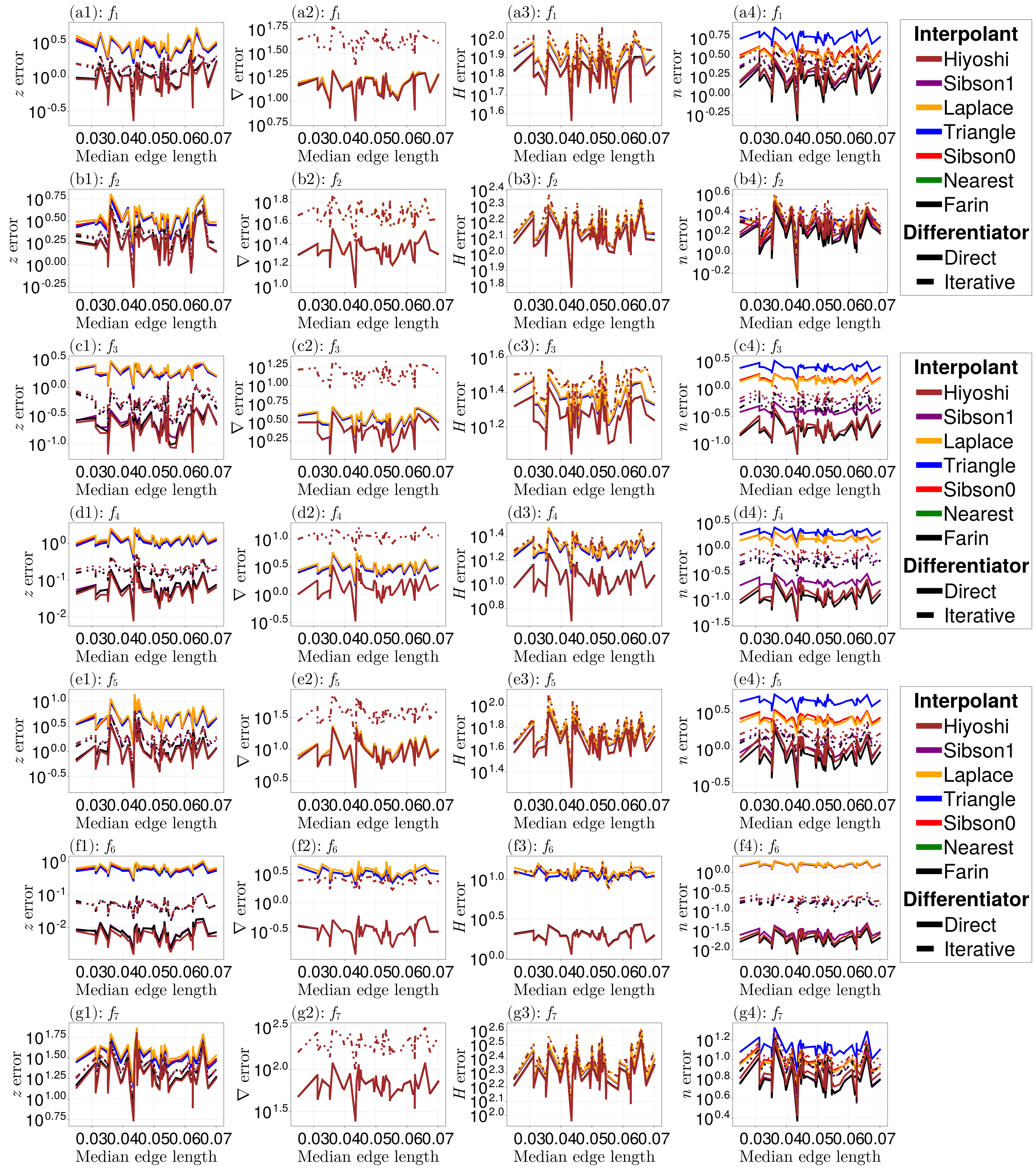
Once again, the Hiyoshi(2) and Farin(1) methods seem preferable, and Direct() seems to have greater results over Iterative().
Computation Times
It is important to note that using the smooth interpolants comes at a cost of greater running time. If $n$ is the number of natural neighbours around a point $\boldsymbol x_0$, then computing $f^{\text{HIY}}(\boldsymbol x_0)$ is about $\mathcal O(n^5)$, and $f^{\text{FAR}}(\boldsymbol x_0)$ is $\mathcal O(n^3)$. Derivative generation also has this complexity when using these interpolants (since it involves solving a least squares problem). Of course, this complexity doesn't typically matter so much since (1) many points are being evaluated at using multithreading and (2) points have, on average, six natural neighbours only in most triangulations.
Let us explore here how long it takes to compute the interpolant as a function of the number of natural neighbours. There are many ways to measure this properly, e.g. collecting large samples of computation times from random data sets, but here we take a simple approach where we construct a triangulation with a point $\boldsymbol x_1 = \boldsymbol 0$ surrounded by $m$ points on a circle. This point $\boldsymbol x_1$ will have approximately $m$ natural neighbours. (Note that we do not care about the number of data points in the dataset since these interpolants are local.) The function we use for this is:
function circular_example(m) # extra points are added outside of the circular barrier for derivative generation
    pts = [(cos(θ) + 1e-6randn(), sin(θ) + 1e-6randn()) for θ = LinRange(0, 2π, (m + 1))][1:end-1] # avoid cocircular points
    extra_pts = NTuple{2, Float64}[]
    while length(extra_pts) < 50
        p = (5randn(), 5randn())
        if norm(p) > 1.01
            push!(extra_pts, p)
        end
    end
    append!(pts, extra_pts)
    tri = triangulate(pts)
    return tri
end
To perform the benchmarks, we use:
function running_time_analysis(itp_method, m_range, g)
    running_times = zeros(length(m_range))
    for (i, m) in enumerate(m_range)
        tri = circular_example(m)
        z = [g(x, y) for (x, y) in DelaunayTriangulation.each_point(tri)]
        itp = interpolate(tri, z; derivatives=true)
        b = @benchmark $itp($0.0, $0.0; method=$itp_method)
        running_times[i] = minimum(b.times) / 1e6 # ms
    end
    return DataFrame(
        running_times = running_times,
        method = itp_alias_map[itp_method],
        m = m_range
    )
end
function running_time_analysis(m_range, g)
    df = DataFrame(
        running_times = Float64[],
        method = Symbol[],
        m = Int[]
    )
    for itp_method in itp_methods
        _running_times = running_time_analysis(itp_method, m_range, g)
        append!(df, _running_times)
    end
    return df
end
Now let us benchmark and plot the results.
m_range = 3:20
g = f[end]
running_times = running_time_analysis(m_range, g)

fig = data(running_times) *
      mapping(:m, :running_times) *
      mapping(color=:method) *
      visual(Scatter, markersize=14) |> plt ->
    draw(plt; axis=(width=600, height=400, yscale=log10, xlabel=L"$ $Number of natural neighbours", ylabel=L"$t$ (ms)"))
vlines!(fig.figure[1, 1], [6], linewidth=3, linestyle=:dash, color=:black)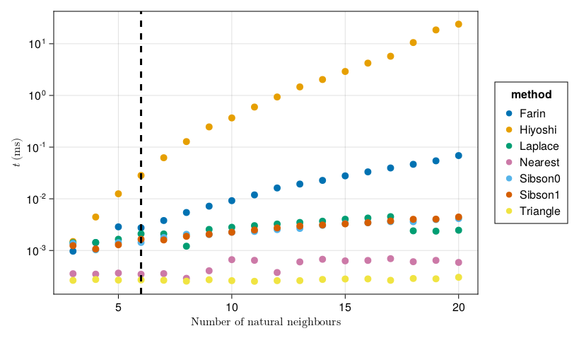
The benchmarks are shown above, with a vertical black line at $m = 6$ (the expected number of neighbours in a triangulation). We see that the Triangle() and Nearest() methods are the fastest, as we'd expect, and are of course independent of $m$. The other methods which are $C^0$ at the data sites, Sibson(0) and Laplace(), are fast and have about the same runtime (both of them essentially perform the same number of operations). When considering smooth interpolants, Sibson(1) is about the same as Sibson(0). The remaining two methods, Farin(1) and Hiyoshi(2), are the slowest as we expect. Hiyoshi(2) can even take more than 10 seconds with 20 natural neighbours (which is not typical, but could happen on real datasets).
Overall, while Hiyoshi(2) seems to be the best interpolant, Farin(1) could probably serve as a better default if you are concerned about runtime and don't need second derivative information.
To give another benchmark, here are some benchmarks where we take a structured triangulation and evaluate the interpolants at $10,000,000$ query points.
x = LinRange(0, 1, 25)
y = LinRange(0, 1, 25)
pts = vec([(x, y) for x in x, y in y])
tri = triangulate(pts)
z = [g(x, y) for (x, y) in DelaunayTriangulation.each_point(tri)]
itp = interpolate(tri, z; derivatives = true)
n = 10_000_000
xq = rand(n)
yq = rand(n)
julia> @time itp(xq, yq; method = Sibson(0));
1.418889 seconds (8.42 k allocations: 76.902 MiB, 0.49% compilation time)
julia> @time itp(xq, yq; method = Triangle());
0.552120 seconds (8.27 k allocations: 76.854 MiB, 1.38% compilation time)
julia> @time itp(xq, yq; method = Nearest());
0.592610 seconds (8.27 k allocations: 76.854 MiB, 1.25% compilation time)
julia> @time itp(xq, yq; method = Laplace());
1.142635 seconds (8.27 k allocations: 76.854 MiB, 0.64% compilation time)
julia> @time itp(xq, yq; method = Sibson(1));
1.498346 seconds (8.27 k allocations: 76.854 MiB, 0.47% compilation time)
julia> @time itp(xq, yq; method = Farin(1));
2.187066 seconds (8.27 k allocations: 76.855 MiB, 0.36% compilation time)
julia> @time itp(xq, yq; method = Hiyoshi(2));
13.762652 seconds (9.26 k allocations: 76.920 MiB, 0.06% compilation time)Conclusion
Overall, the smooth interpolants have the best performance, with Farin(1) and Hiyoshi(2) typically beating most interpolants. Hiyoshi(2) is much slower than the other interpolants, though, and Farin(1) may be a preferable interpolant if $C^1$ continuity at the data sites is sufficient. For generating derivatives, the Direct() seems to beat the results with the Iterative() method in most situations.