Switzerland Elevation Data
Here we consider a more involved example, constructing an interpolant over elevation data of Switzerland. We use data from geoBoundaries who credits OpenStreetMap for the data (available under an Open Database License). The data is available as a gist, which was generated with the following R code (you don't need to run this code - we will download it directly from the gist soon):
## Install and load the packages
#install.packages(c("remotes", "sf", "raster", "elevatr", "dplyr", "magrittr"))
#install.packages(c("dplyr", "magrittr"))
#remotes::install_gitlab("dickoa/rgeoboundaries")
library(rgeoboundaries)
library(sf)
library(raster)
library(elevatr)
#library(dplyr)
#library(magrittr)

## Get the elevation and polygon data
swiss_bound <- rgeoboundaries::geoboundaries("Switzerland")
elevation_data_rast <- elevatr::get_elev_raster(locations = swiss_bound, z = 7, clip = "locations")
boundary_coords <- rasterToPolygons(elevation_data_rast > -Inf, dissolve = TRUE) # https://gis.stackexchange.com/a/187800
elevation_data_xy <- as.data.frame(elevation_data_rast, xy = TRUE)
colnames(elevation_data_xy)[3] <- "elevation"
elevation_data_xy <- elevation_data_xy[complete.cases(elevation_data_xy), ]
all_polygons = boundary_coords@polygons[[1]]@Polygons

## Inspect all the polygons
#conv = function(polygon, id) {
#  coords = polygon@coords
#  dir = polygon@ringDir
#  hole = polygon@hole
#  df = tibble(x = coords[, 1], y = coords[, 1], dir = polygon@ringDir, hole = polygon@hole, id = id)
#}
#polygon_df = vector('list', length(all_polygons))
#for (i in seq_along(polygon_df)) {
#  polygon_df[[i]] = conv(all_polygons[[i]], i)
#}
#polygon_df %<>% bind_rows(.id = "column_label")
# ^ After inspecting these results, the only polygon of interest is the first one.

polygons = all_polygons[[1]]@coords
x = elevation_data_xy[, 1]
y = elevation_data_xy[, 2]
z = elevation_data_xy[, 3]
bnd_x = polygons[, 1]
bnd_y = polygons[, 2]
For this example, load the following packages:
using NaturalNeighbours
using CairoMakie
using DelaunayTriangulation
using DelimitedFiles
using Downloads
using StableRNGs
using StatsBase
Downloading the Data
To start, let us download and setup the data. We need to get the data sites, the elevation values, and also the boundary points.
data_url = "https://gist.githubusercontent.com/DanielVandH/13687b0918e45a416a5c93cd52c91449/raw/a8da6cdc94859fd66bcff85a2307f0f9cd57a18c/data.txt"
boundary_url = "https://gist.githubusercontent.com/DanielVandH/13687b0918e45a416a5c93cd52c91449/raw/a8da6cdc94859fd66bcff85a2307f0f9cd57a18c/boundary.txt"
data_dir = Downloads.download(data_url)
boundary_dir = Downloads.download(boundary_url)
data = readdlm(data_dir, skipstart=6)
data[:, 3] ./= 1000.0 # m -> km
boundary = readdlm(boundary_dir, skipstart=6)
good_elevation = findall(≥(0), @view data[:, 3])
data = @views data[good_elevation, :]
data_sites = [(data[i, 1], data[i, 2]) for i in axes(data, 1)]
elevation_data = @views data[:, 3]
boundary_points = [(boundary[i, 1], boundary[i, 2]) for i in axes(boundary, 1)]
Downsampling and Setting up the Data for Plotting
We now setup the data for plotting. We want to use tricontourf!, so we need to get a triangulation of the data. Since the boundary_points do not actually store a subset of the points from data_sites, we can't just do e.g. indexin(boundary_points, data_sites) to get the associated boundary indices, so we instead find the closest data site to each boundary point.
function nearest_tuple(q, data)
    δ = Inf
    nearest_idx = 0
    qx, qy = getxy(q)
    for (i, p) in pairs(data)
        px, py = getxy(p)
        δ₁ = (qx - px)^2 + (qy - py)^2
        if δ₁ < δ
            δ = δ₁
            nearest_idx = i
        end
    end
    return nearest_idx
end
function update_boundary(boundary_points, data_sites)
    boundary_nodes = map(q -> nearest_tuple(q, data_sites), boundary_points)
    unique!(boundary_nodes)
    push!(boundary_nodes, boundary_nodes[begin])
    reverse!(boundary_nodes) # so that the boundary is traversed clockwise
    boundary_points = data_sites[boundary_nodes]
    return boundary_points, data_sites, boundary_nodes
end
boundary_points, data_sites, boundary_nodes = update_boundary(boundary_points, data_sites)
Next, before, we plot, let us downsample the data. We do this since the data set is quite large, so when we interpolate it'll be useful to have fewer data points for the purpose of this example.
rng = StableRNG(123)
desample_idx = sample(rng, axes(data, 1), 5000, replace=false)
ds_data = data[desample_idx, :]
ds_data_sites = [(ds_data[i, 1], ds_data[i, 2]) for i in axes(ds_data, 1)]
ds_elevation_data = @views ds_data[:, 3]
ds_boundary_points, ds_data_sites, ds_boundary_nodes = update_boundary(boundary_points, ds_data_sites)
reverse!(ds_boundary_nodes) # so that the boundary is traversed clockwise
ds_tri = triangulate(ds_data_sites, boundary_nodes=ds_boundary_nodes)
ds_triangles = [T[j] for T in each_solid_triangle(ds_tri), j in 1:3]
Looking at the Data
Now let's look at the data.
colorrange = (0, 4)
levels = LinRange(colorrange..., 40)
fig = Figure(fontsize=24)
ax1 = Axis3(fig[1, 1], xlabel="Longitude", ylabel="Latitude", zlabel="Elevation (km)", width=600, height=400, azimuth=0.9, title="(c): Downsampled height data (n = $(length(ds_elevation_data)))", titlealign=:left)
mesh!(ax1, ds_data, ds_triangles, color=ds_elevation_data, colorrange=colorrange)
ax2 = Axis(fig[1, 2], xlabel="Longitude", ylabel="Latitude", width=600, height=400, title="(d): Downsampled height data (n = $(length(ds_elevation_data)))", titlealign=:left)
tf = tricontourf!(ax2, ds_tri, ds_elevation_data, levels=levels)
Colorbar(fig[1:2, 3], tf)
resize_to_layout!(fig)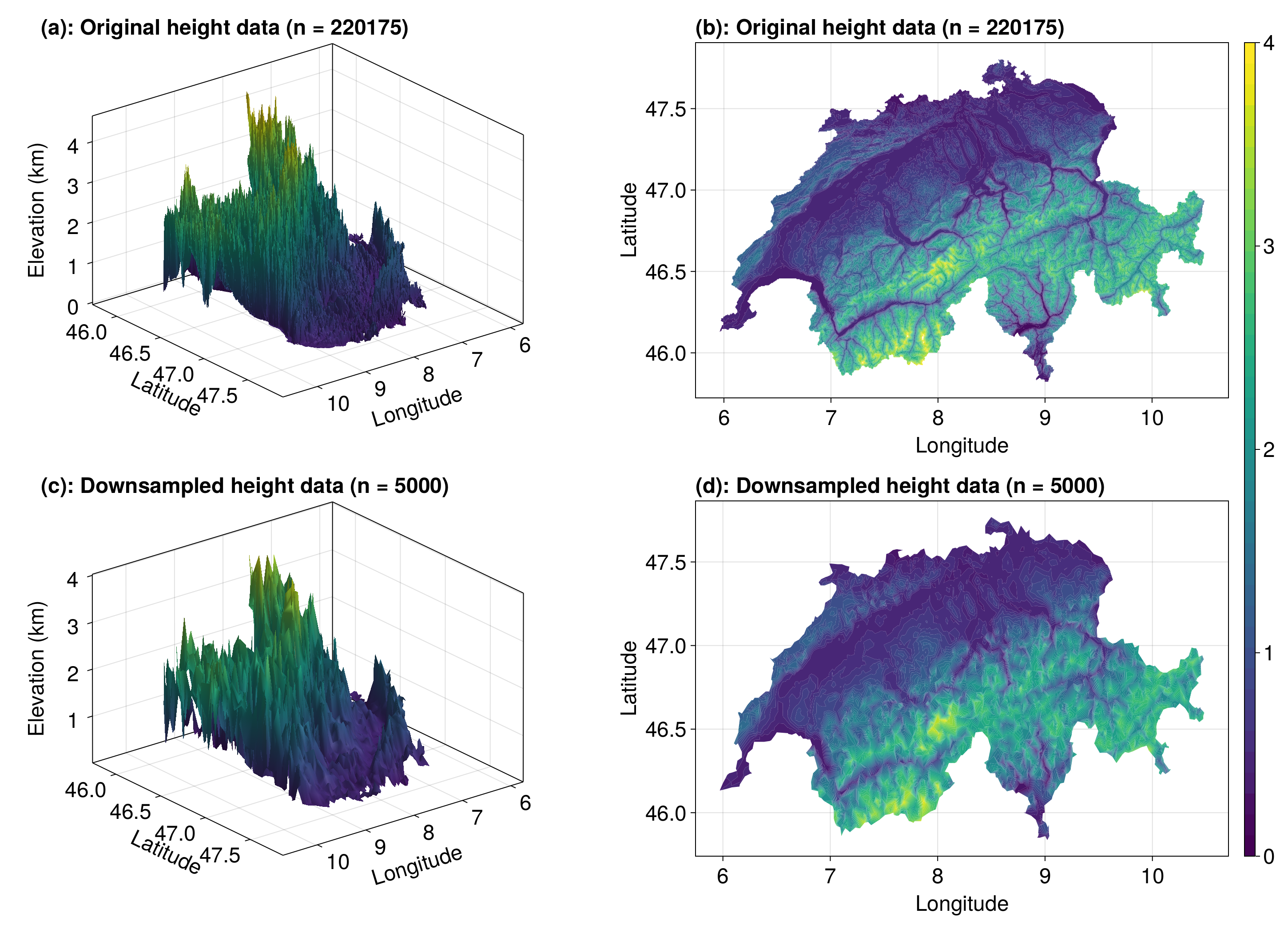
We see that the downsampled data isn't that much different, despite having $n = 5,000$ points rather than $n = 220,175$ as in the original data set. Of course, the boundary has been trimmed a bit (if we really cared, we probably wouldn't have downsampled the boundary, but instead only downsampled the interior points - not relevant for this example).
Interpolating
Now let's define and evaluate our interpolant.
## Define the interpolant
interpolant = interpolate(ds_data_sites, ds_elevation_data; derivatives=true)

## Evaluate the interpolant
a, b, c, d = DelaunayTriangulation.polygon_bounds(ds_data_sites, ds_boundary_nodes)
nx = 250
ny = 250
xg = LinRange(a, b, nx)
yg = LinRange(c, d, ny)
x = [xg[i] for i in 1:nx, j in 1:ny] |> vec
y = [yg[j] for i in 1:nx, j in 1:ny] |> vec

sibson_vals = interpolant(x, y; method=Sibson(), parallel=true)
sibson_1_vals = interpolant(x, y; method=Sibson(1), parallel=true)
laplace_vals = interpolant(x, y; method=Laplace(), parallel=true)
triangle_vals = interpolant(x, y; method=Triangle(), parallel=true)
nearest_vals = interpolant(x, y; method=Nearest(), parallel=true)
farin_vals = interpolant(x, y; method=Farin(), parallel=true)
hiyoshi_vals = interpolant(x, y; method=Hiyoshi(2), parallel=true)
Let's look at our results for each of these methods.
query_tri = triangulate([x'; y']; randomise=false)
query_triangles = [T[j] for T in each_solid_triangle(query_tri), j in 1:3]
function plot_results!(fig, i1, j1, i2, j2, x, y, xg, yg, vals, title1, title2, query_triangles, query_tri, a, b, c, d, e, f, nx, ny)
    ax = Axis3(fig[i1, j1], xlabel="Longitude", ylabel="Latitude", zlabel="Elevation (km)", width=600, height=400, azimuth=0.9, title=title1, titlealign=:left)
    m = mesh!(ax, hcat(x, y, vals), query_triangles, color=vals, colorrange=colorrange)
    xlims!(ax, a, b)
    ylims!(ax, c, d)
    zlims!(ax, e, f)
    ax = Axis(fig[i2, j2], xlabel="Longitude", ylabel="Latitude", width=600, height=400, title=title2, titlealign=:left)
    contourf!(ax, xg, yg, reshape(vals, (nx, ny)), levels=levels)
    lines!(ax, [get_point(query_tri, i) for i in get_convex_hull_vertices(query_tri)], color=:red, linewidth=4, linestyle=:dash)
    lines!(ax, ds_boundary_points, color=:white, linewidth=4)
    xlims!(ax, a, b)
    ylims!(ax, c, d)
    return m
end
function plot_results(sibson_vals, sibson_1_vals, laplace_vals, triangle_vals, nearest_vals, farin_vals, hiyoshi_vals, query_triangles, interpolant, a, b, c, d, e, f, nx, ny, data, triangles, elevation_data, tri)
    fig = Figure(fontsize=24)
    m1 = plot_results!(fig, 1, 1, 1, 2, x, y, xg, yg, sibson_vals, "(a): Sibson", "(b): Sibson", query_triangles, interpolant.triangulation, a, b, c, d, e, f, nx, ny)
    m2 = plot_results!(fig, 1, 3, 1, 4, x, y, xg, yg, sibson_1_vals, "(c): Sibson-1", "(d): Sibson-1", query_triangles, interpolant.triangulation, a, b, c, d, e, f, nx, ny)
    m3 = plot_results!(fig, 2, 1, 2, 2, x, y, xg, yg, laplace_vals, "(e): Laplace", "(f): Laplace", query_triangles, interpolant.triangulation, a, b, c, d, e, f, nx, ny)
    m4 = plot_results!(fig, 2, 3, 2, 4, x, y, xg, yg, triangle_vals, "(g): Triangle", "(h): Triangle", query_triangles, interpolant.triangulation, a, b, c, d, e, f, nx, ny)
    m5 = plot_results!(fig, 3, 1, 3, 2, x, y, xg, yg, nearest_vals, "(i): Nearest", "(j): Nearest", query_triangles, interpolant.triangulation, a, b, c, d, e, f, nx, ny)
    m6 = plot_results!(fig, 3, 3, 3, 4, x, y, xg, yg, farin_vals, "(k): Farin", "(ℓ): Farin", query_triangles, interpolant.triangulation, a, b, c, d, e, f, nx, ny)
    m7 = plot_results!(fig, 4, 1, 4, 2, x, y, xg, yg, hiyoshi_vals, "(m): Hiyoshi", "(n): Hiyoshi", query_triangles, interpolant.triangulation, a, b, c, d, e, f, nx, ny)
    ax = Axis3(fig[4, 3], xlabel="Longitude", ylabel="Latitude", zlabel="Elevation (km)", width=600, height=400, azimuth=0.9, title="(k): Original height data", titlealign=:left)
    mesh!(ax, data, triangles, color=elevation_data, colorrange=(0, 4))
    xlims!(ax, a, b)
    ylims!(ax, c, d)
    zlims!(ax, e, f)
    ax = Axis(fig[4, 4], xlabel="Longitude", ylabel="Latitude", width=600, height=400, title="(o): Original height data", titlealign=:left)
    tricontourf!(ax, tri, elevation_data, levels=levels)
    xlims!(ax, a, b)
    ylims!(ax, c, d)
    Colorbar(fig[1:4, 5], m1)
    resize_to_layout!(fig)
    return fig
end
e, f = 0.0, 4.5
fig = plot_results(sibson_vals, sibson_1_vals, laplace_vals, triangle_vals, nearest_vals, farin_vals, hiyoshi_vals, query_triangles, interpolant, a, b, c, d, e, f, nx, ny, ds_data, ds_triangles, ds_elevation_data, ds_tri)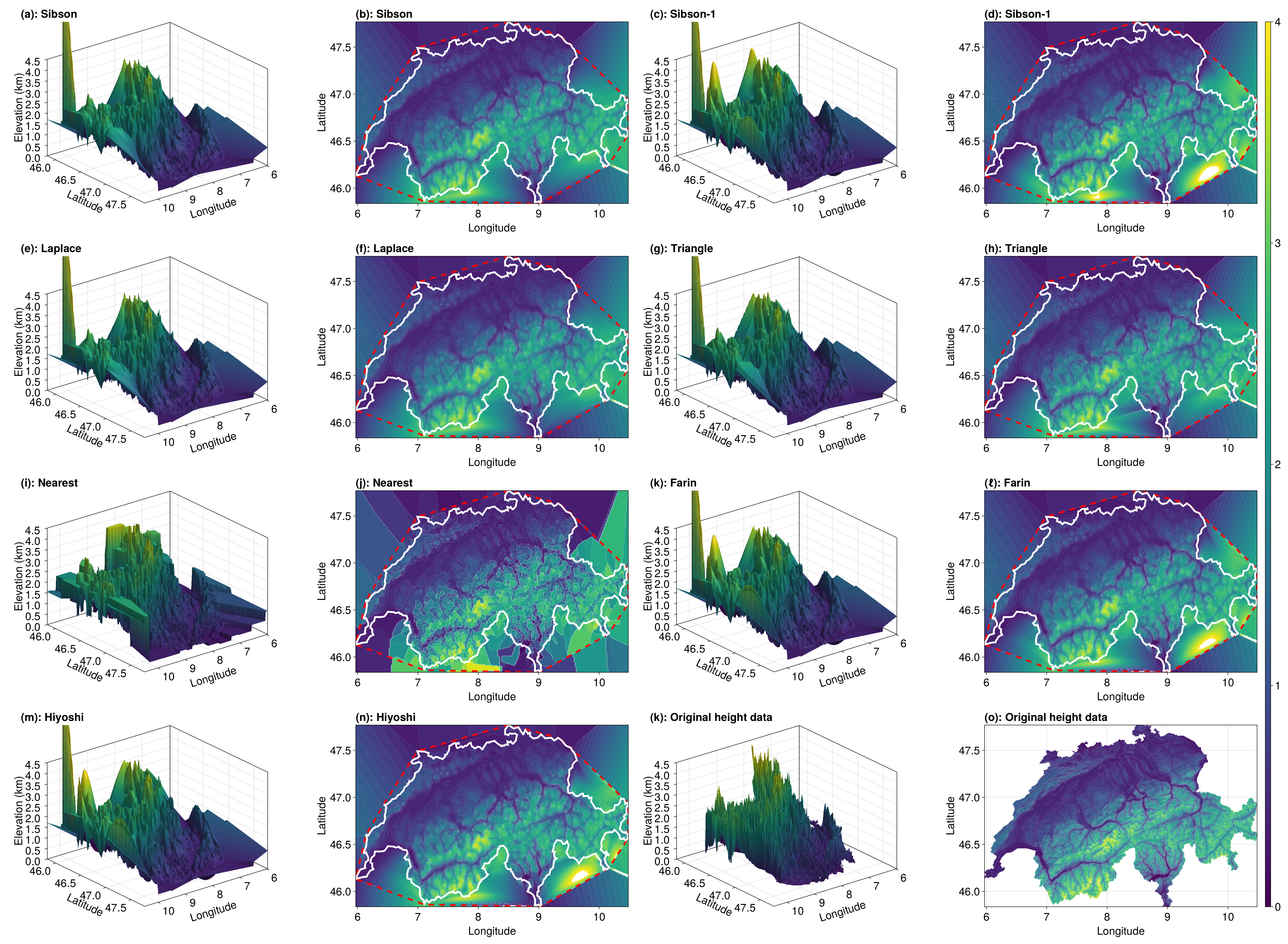
We see that the results are pretty similar across the methods except for Nearest(). We could compute the errors between the interpolant and the points that we removed from the dataset to quantify this better, but we won't do that –- we're not intending to a comprehensive analysis here.
Eliminating Points Outside of the Convex Hull
One issue with the interpolant is that the extrapolated results are distracting. Let's set project=false to remove values outside of the convex hull of our data sites.
sibson_vals_p = interpolant(x, y; method=Sibson(), parallel=true, project=false)
sibson_1_vals_p = interpolant(x, y; method=Sibson(1), parallel=true, project=false)
laplace_vals_p = interpolant(x, y; method=Laplace(), parallel=true, project=false)
triangle_vals_p = interpolant(x, y; method=Triangle(), parallel=true, project=false)
nearest_vals_p = interpolant(x, y; method=Nearest(), parallel=true, project=false)
farin_vals_p = interpolant(x, y; method=Farin(), parallel=true, project=false)
hiyoshi_vals_p = interpolant(x, y; method=Hiyoshi(2), parallel=true, project=false)
fig = plot_results(sibson_vals_p, sibson_1_vals_p, laplace_vals_p, triangle_vals_p, nearest_vals_p, farin_vals_p, hiyoshi_vals_p, query_triangles, interpolant, a, b, c, d, e, f, nx, ny, ds_data, ds_triangles, ds_elevation_data, ds_tri)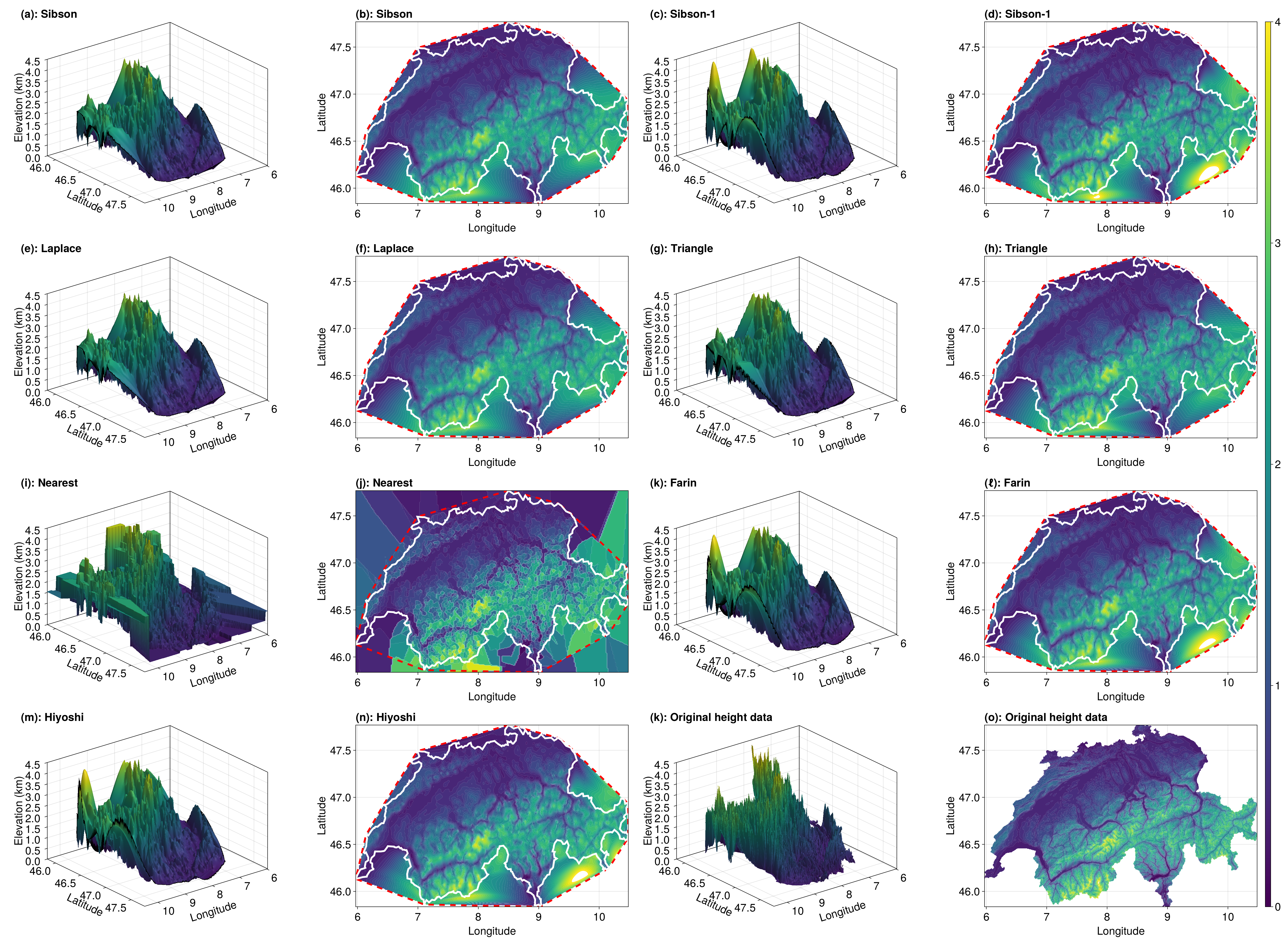
Of course, this is still not perfect because Switzerland is not convex! There's still points being extrapolated, and we have to handle this manually.
Eliminating Points Outside of Switzerland
The function we need is identify_exterior_points, which we use together with a representation of the boundary of Switzerland (hence why we got the boundary nodes earlier). We replace all exterior values with Inf so that they don't get plotted (using NaN leads to issues with surface!'s shading for some reason).
exterior_idx = identify_exterior_points(x, y, ds_data_sites, ds_boundary_nodes)
sibson_vals_p[exterior_idx] .= Inf
sibson_1_vals_p[exterior_idx] .= Inf
laplace_vals_p[exterior_idx] .= Inf
triangle_vals_p[exterior_idx] .= Inf
nearest_vals_p[exterior_idx] .= Inf
farin_vals_p[exterior_idx] .= Inf
hiyoshi_vals_p[exterior_idx] .= Inf
fig = plot_results(sibson_vals_p, sibson_1_vals_p, laplace_vals_p, triangle_vals_p, nearest_vals_p, farin_vals_p, hiyoshi_vals_p, query_triangles, interpolant, a, b, c, d, e, f, nx, ny, ds_data, ds_triangles, ds_elevation_data, ds_tri)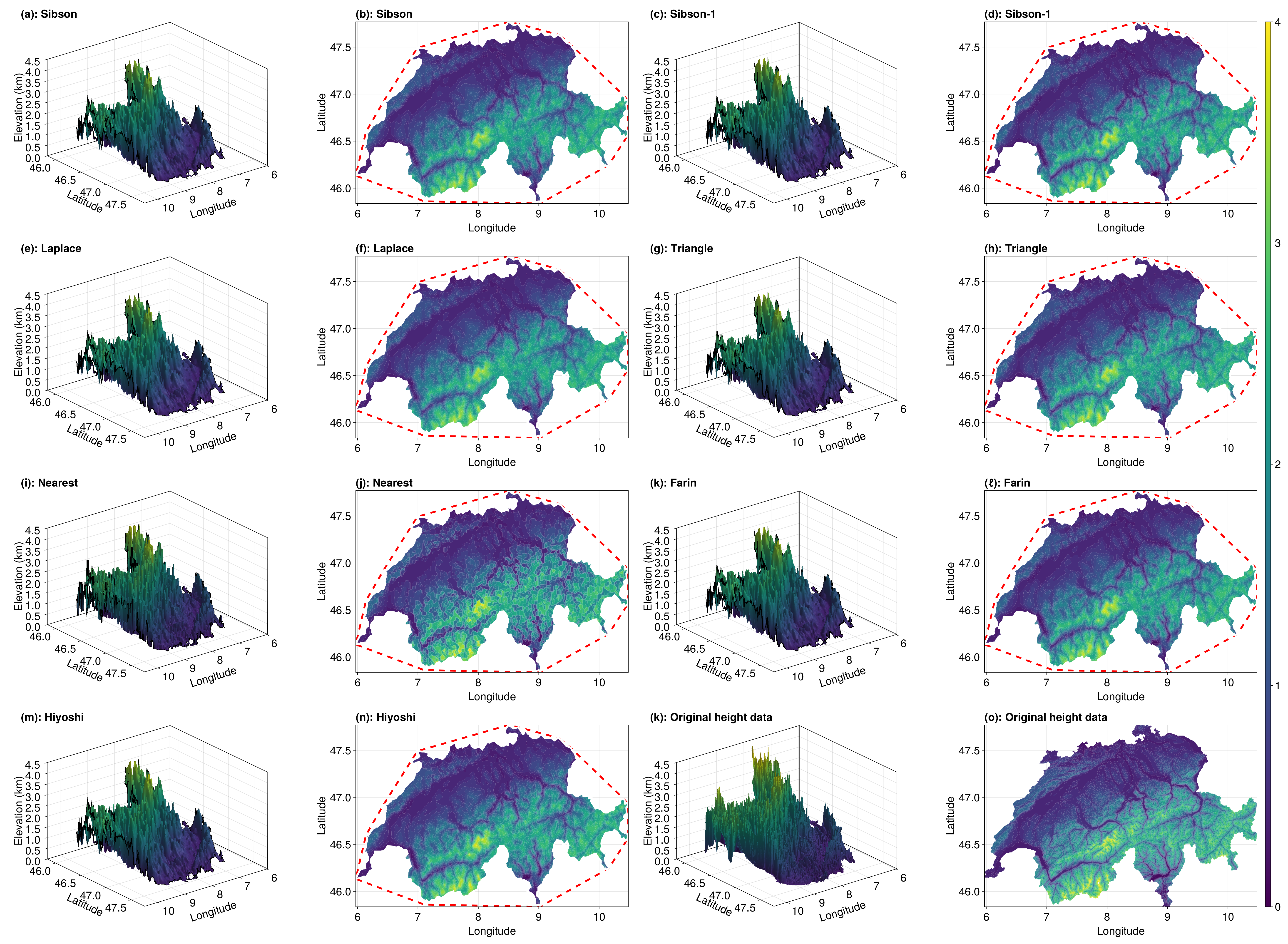
Perfect!