Interpolation Example
Let us give an example of how interpolation can be performed. We consider the function
\[f(x, y) = \frac19\left[\tanh\left(9y-9x\right) + 1\right].\]
First, let us generate some data.
using NaturalNeighbours
using CairoMakie
using StableRNGs

f = (x, y) -> (1 / 9) * (tanh(9 * y - 9 * x) + 1)

rng = StableRNG(123)
x = rand(rng, 100)
y = rand(rng, 100)
z = f.(x, y)
We can now construct our interpolant. To use the Sibson-1 interpolant, we need to have gradient information, so we specify derivatives=true to make sure these get generated at the data sites.
itp = interpolate(x, y, z; derivatives=true)This itp is now callable. Let's generate a grid to evaluate itp at.
xg = LinRange(0, 1, 100)
yg = LinRange(0, 1, 100)
_x = vec([x for x in xg, _ in yg])
_y = vec([y for _ in xg, y in yg])
We use vectors for this evaluation rather than evaluating like, say, [itp(x, y) for x in xg, y in yg], since itp's evaluation will use multithreading if we give it vectors. Consider the following times (including the time to make the vectors in the vector case):
using BenchmarkTools
function testf1(itp, xg, yg, parallel)
    _x = vec([x for x in xg, _ in yg])
    _y = vec([y for _ in xg, y in yg])
    return itp(_x, _y; parallel=parallel)
end
testf2(itp, xg, yg) = [itp(x, y) for x in xg, y in yg]
b1 = @benchmark $testf1($itp, $xg, $yg, $true)
b2 = @benchmark $testf2($itp, $xg, $yg)
b3 = @benchmark $testf1($itp, $xg, $yg, $false)
julia> b1
BenchmarkTools.Trial: 2310 samples with 1 evaluation.
Range (min … max): 1.333 ms … 165.550 ms ┊ GC (min … max): 0.00% … 98.28%
Time (median): 1.781 ms ┊ GC (median): 0.00%
Time (mean ± σ): 2.155 ms ± 3.446 ms ┊ GC (mean ± σ): 3.27% ± 2.04%
▄▆█▄▁
▂▂▄▃▅▆█████▆▅▃▃▂▂▂▂▂▂▂▃▂▂▃▃▃▃▃▃▄▃▄▄▄▄▅▅▄▄▄▄▄▃▃▃▄▃▂▂▂▂▁▂▁▁▁▁ ▃
1.33 ms Histogram: frequency by time 3.33 ms <
Memory estimate: 254.33 KiB, allocs estimate: 146.
julia> b2
BenchmarkTools.Trial: 257 samples with 1 evaluation.
Range (min … max): 14.790 ms … 27.120 ms ┊ GC (min … max): 0.00% … 0.00%
Time (median): 18.136 ms ┊ GC (median): 0.00%
Time (mean ± σ): 19.531 ms ± 4.177 ms ┊ GC (mean ± σ): 0.00% ± 0.00%
▅█
▆██▄▄▄▄▂▅▁▁▄▃▄▅▃▃▃▃▁▃▃▁▃▄▃▃▃▂▂▄▂▃▃▂▄▂▄▄▃▂▄▄▃▃▄▃▄▄▃▄▃▃▄▄▂▄▅▄ ▃
14.8 ms Histogram: frequency by time 26.7 ms <
Memory estimate: 78.17 KiB, allocs estimate: 2.
julia> b3
BenchmarkTools.Trial: 267 samples with 1 evaluation.
Range (min … max): 14.986 ms … 27.264 ms ┊ GC (min … max): 0.00% … 0.00%
Time (median): 17.354 ms ┊ GC (median): 0.00%
Time (mean ± σ): 18.710 ms ± 3.750 ms ┊ GC (mean ± σ): 0.00% ± 0.00%
▄█
▄██▇▄▃▃▄▃▃▃▃▃▃▃▄▄▂▃▃▃▃▃▃▃▃▃▃▃▃▂▁▃▃▃▃▃▃▃▃▃▂▃▃▂▃▃▂▂▁▂▃▃▂▃▂▃▄▃ ▃
15 ms Histogram: frequency by time 26.7 ms <
Memory estimate: 234.67 KiB, allocs estimate: 10.See that itp(_x, _y) took about 1.3 ms, while the latter two approaches both take around 15 ms. Pretty impressive given that we are evaluating $100^2$ points - this is a big advantage of local interpolation making parallel evaluation so cheap and simple. This effect can be made even more clear if we use more points:
xg = LinRange(0, 1, 1000)
yg = LinRange(0, 1, 1000)
b1 = @benchmark $testf1($itp, $xg, $yg, $true)
b2 = @benchmark $testf2($itp, $xg, $yg)
b3 = @benchmark $testf1($itp, $xg, $yg, $false)
julia> b1
BenchmarkTools.Trial: 27 samples with 1 evaluation.
Range (min … max): 132.766 ms … 354.348 ms ┊ GC (min … max): 0.00% … 0.00%
Time (median): 144.794 ms ┊ GC (median): 0.00%
Time (mean ± σ): 188.429 ms ± 79.396 ms ┊ GC (mean ± σ): 0.37% ± 2.38%
▁█▃▁
████▄▄▄▁▁▁▁▁▁▄▁▁▁▁▁▁▁▁▁▁▁▁▁▁▁▁▁▁▁▁▁▁▄▁▁▁▁▄▄▁▁▁▁▁▁▁▁▄▁▁▁▁▁▁▁▄▇ ▁
133 ms Histogram: frequency by time 354 ms <
Memory estimate: 22.91 MiB, allocs estimate: 157.
julia> b2
BenchmarkTools.Trial: 2 samples with 1 evaluation.
Range (min … max): 2.564 s … 2.794 s ┊ GC (min … max): 0.00% … 0.00%
Time (median): 2.679 s ┊ GC (median): 0.00%
Time (mean ± σ): 2.679 s ± 162.574 ms ┊ GC (mean ± σ): 0.00% ± 0.00%
█ █
█▁▁▁▁▁▁▁▁▁▁▁▁▁▁▁▁▁▁▁▁▁▁▁▁▁▁▁▁▁▁▁▁▁▁▁▁▁▁▁▁▁▁▁▁▁▁▁▁▁▁▁▁▁▁▁▁█ ▁
2.56 s Histogram: frequency by time 2.79 s <
Memory estimate: 7.63 MiB, allocs estimate: 2.
julia> b3
BenchmarkTools.Trial: 2 samples with 1 evaluation.
Range (min … max): 2.557 s … 2.624 s ┊ GC (min … max): 0.00% … 0.00%
Time (median): 2.590 s ┊ GC (median): 0.00%
Time (mean ± σ): 2.590 s ± 46.978 ms ┊ GC (mean ± σ): 0.00% ± 0.00%
█ █
█▁▁▁▁▁▁▁▁▁▁▁▁▁▁▁▁▁▁▁▁▁▁▁▁▁▁▁▁▁▁▁▁▁▁▁▁▁▁▁▁▁▁▁▁▁▁▁▁▁▁▁▁▁▁▁█ ▁
2.56 s Histogram: frequency by time 2.62 s <
Memory estimate: 22.89 MiB, allocs estimate: 10.Now let's continue with the example. We compare Sibson-0 to Sibson-1 (going back to the original definitions of xg and yg with $100^2$ points):
sib_vals = itp(_x, _y)
sib1_vals = itp(_x, _y; method=Sibson(1))
Now we can plot.
function plot_itp(fig, x, y, vals, title, i, show_data_sites, itp, xd=nothing, yd=nothing, show_3d=true, levels=-0.1:0.05:0.3)
    ax = Axis(fig[1, i], xlabel="x", ylabel="y", width=600, height=600, title=title, titlealign=:left)
    c = contourf!(ax, x, y, vals, colormap=:viridis, levels=levels, extendhigh=:auto)
    show_data_sites && scatter!(ax, xd, yd, color=:red, markersize=9)
    tri = itp.triangulation
    ch_idx = get_convex_hull_vertices(tri)
    lines!(ax, [get_point(tri, i) for i in ch_idx], color=:white, linewidth=4)
    if show_3d
        ax = Axis3(fig[2, i], xlabel="x", ylabel="y", zlabel=L"z", width=600, height=600, title=" ", titlealign=:left, azimuth=0.49)
        surface!(ax, x, y, vals, color=vals, colormap=:viridis, colorrange=(-0.1, 0.3))
        zlims!(ax, 0, 0.25)
    end
    return c
end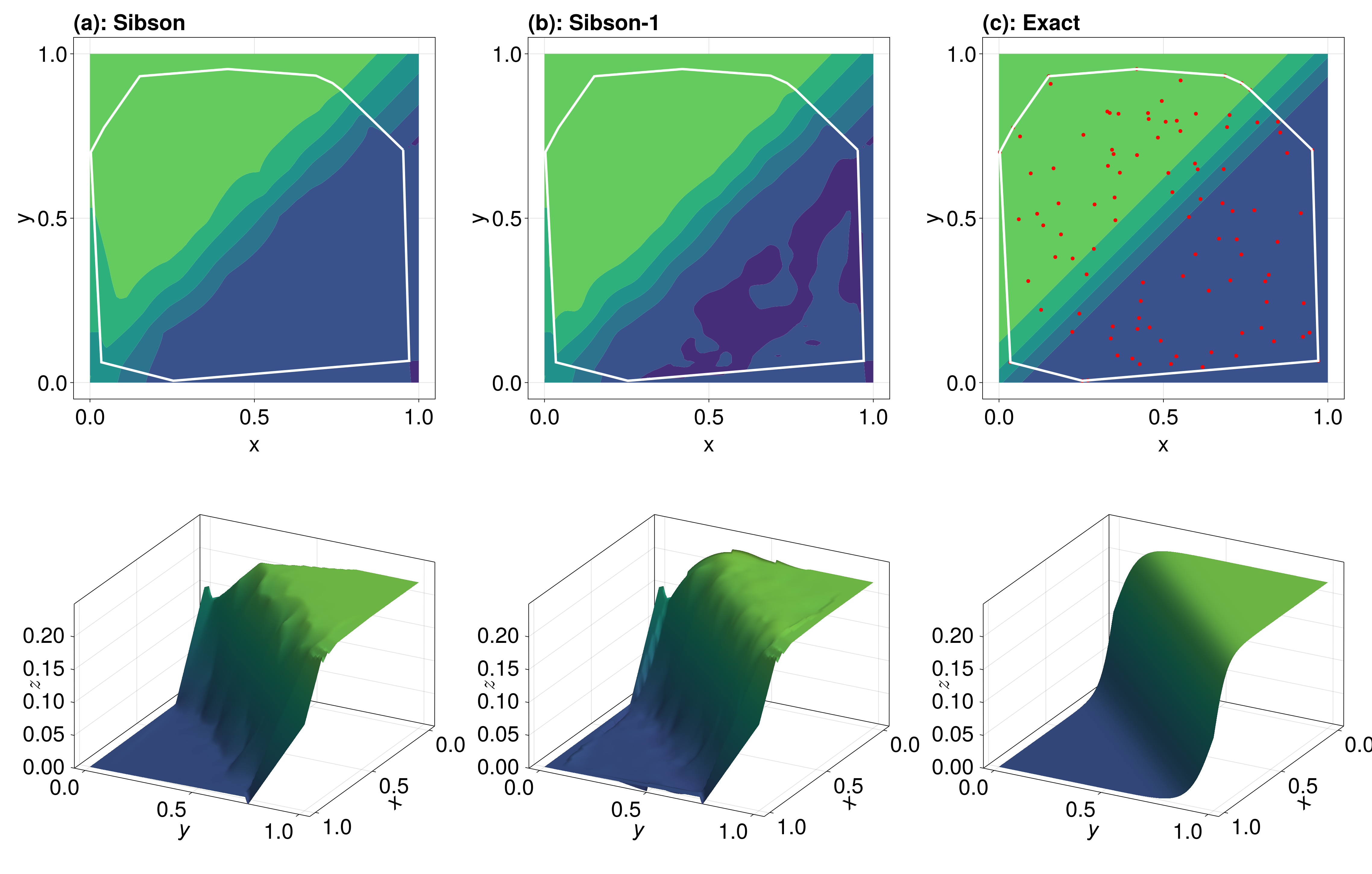
The red points in (c) show the data used for interpolating. The results are pretty similar, although Sibson-1 is more bumpy in the zero region of the function. Sibson-1 is smooth wave on the rising front of the function.
Note that we are extrapolating in some parts of this function, where extrapolation refers to evaluating outside of the convex hull of the data sites. This convex hull is shown in white above. If we wanted to avoid extrapolating entirely, you can use project=false which replaces any extrapolated values with Inf.
sib_vals = itp(_x, _y, project=false)
sib1_vals = itp(_x, _y; method=Sibson(1), project=false)
fig = Figure(fontsize=36)
plot_itp(fig, _x, _y, sib_vals, "(a): Sibson", 1, false, itp, x, y)
plot_itp(fig, _x, _y, sib1_vals, "(b): Sibson-1", 2, false, itp, x, y)
plot_itp(fig, _x, _y, f.(_x, _y), "(c): Exact", 3, true, itp, x, y)
resize_to_layout!(fig)
fig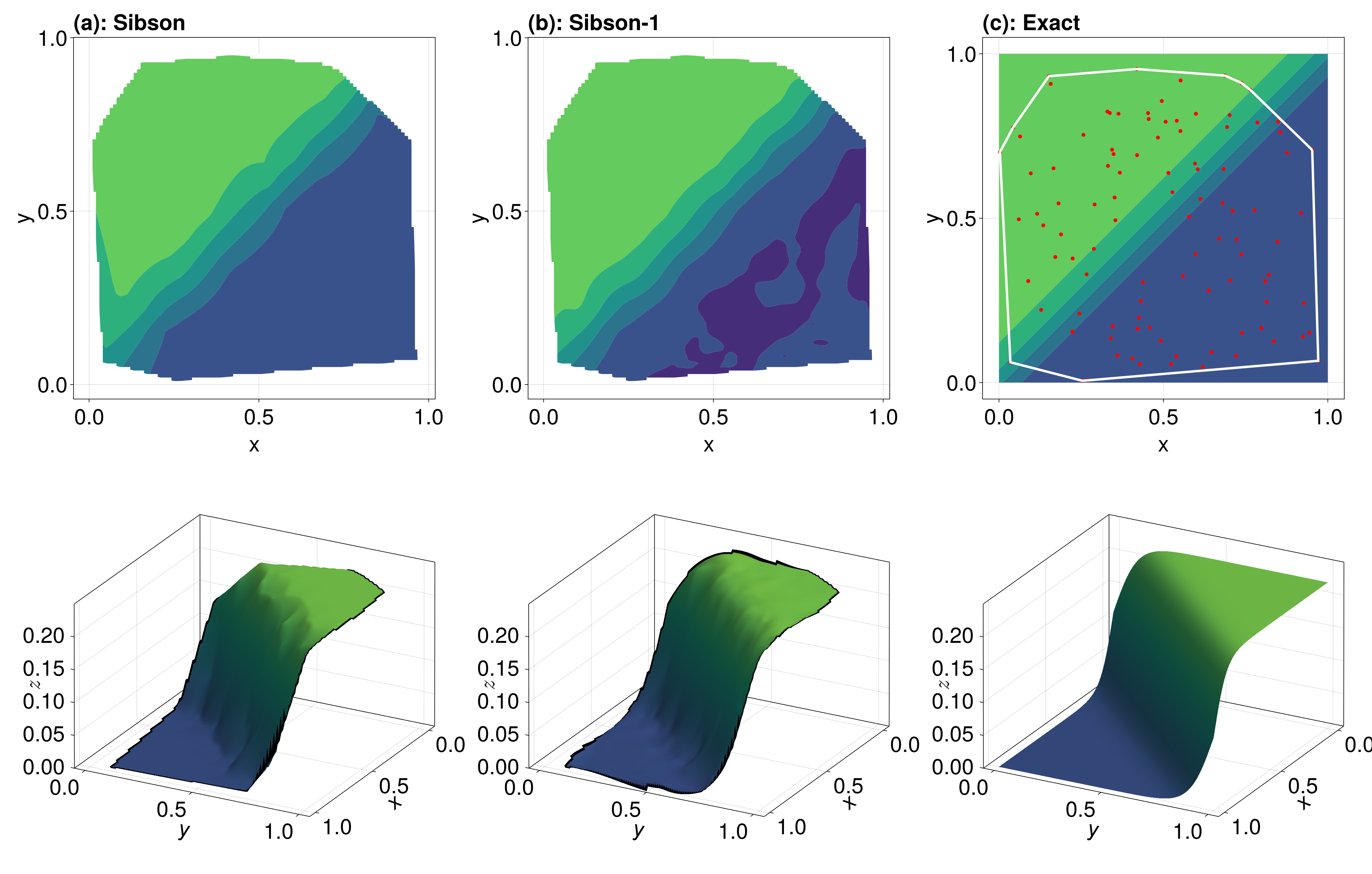
To get a better comparison of the two interpolants, lets plot the errors at each point, including extrapolation.
sib_vals = itp(_x, _y)
sib1_vals = itp(_x, _y; method=Sibson(1))
sib_errs = @. 100abs(sib_vals - f(_x, _y))
sib1_errs = @. 100abs(sib1_vals - f(_x, _y))

fig = Figure(fontsize=36)
plot_itp(fig, _x, _y, sib_errs, "(a): Sibson", 1, true, itp, x, y, false, 0:0.5:3)
c = plot_itp(fig, _x, _y, sib1_errs, "(b): Sibson-1", 2, true, itp, x, y, false, 0:0.5:3)
Colorbar(fig[1, 3], c)
resize_to_layout!(fig)
fig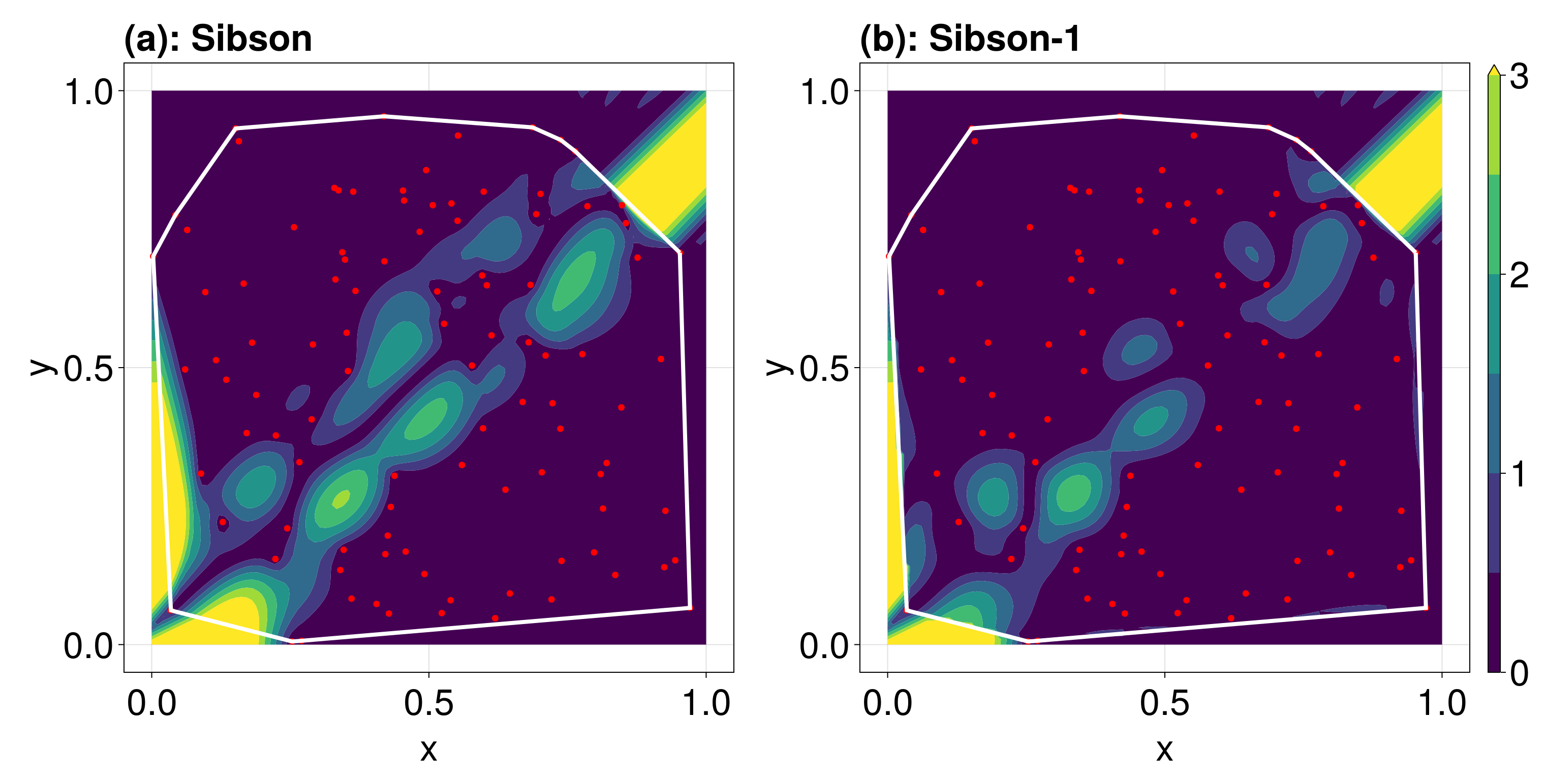
We see that the Sibson-1 interpolant has less error overall. To summarise these errors into a single scalar, we can use the relative root mean square error, defined by
\[\varepsilon_{\text{rrmse}}(\boldsymbol y, \hat{\boldsymbol y}) = 100\sqrt{\frac{\sum_i (y_i - \hat y_i)^2}{\sum_i \hat y_i^2}}.\]
julia> esib0 = 100sqrt(sum((sib_vals .- f.(_x, _y)).^2) / sum(sib_vals.^2))
8.272516151708604

julia> esib1 = 100sqrt(sum((sib1_vals .- f.(_x, _y)).^2) / sum(sib_vals.^2))
6.974149853003652