Differentiation
In this section, we give some of the mathematical detail used for implementing derivative generation, following this thesis. The discussion that follows is primarily sourced from Chapter 6 of the linked thesis. While it is possible to generate derivatives of arbitrary order, our discussion here in this section will be limited to gradient and Hessian generation. These ideas are implemented by the generate_gradients and generate_derivatives functions, which you should use via the differentiate function.
Generation at Data Sites
Let us first consider generating derivatives at the data points used to define the interpolant, $(\boldsymbol x_1, z_1), \ldots, (\boldsymbol x_n, z_n)$. We consider generating the derivatives at a data site $\boldsymbol x_0$, where $\boldsymbol x_0$ is some point in $(\boldsymbol x_1,\ldots,\boldsymbol x_n)$ so that we also know $z_0$.
Direct Generation
Let us consider a direct approach first. In this approach, we generate gradients and Hessians jointly. We approximate the underlying function $f$ by a Taylor series expansion,
\[\tilde f(\boldsymbol x) = z_0 + \tilde f_1(\boldsymbol x) + \tilde f_2(\boldsymbol x) + \tilde f_3(\boldsymbol x),\]
where
\[\begin{align*} \tilde f_1(\boldsymbol x) &= \frac{\partial f(\boldsymbol x_0)}{\partial x}(x-x_0) + \frac{\partial f(\boldsymbol x_0)}{\partial y}(y - y_0), \\ \tilde f_2(\boldsymbol x) &= \frac12\frac{\partial^2 f(\boldsymbol x_0)}{\partial x^2}(x - x_0)^2 + \frac12{\partial^2 f(\boldsymbol x_0)}{\partial y^2}(y - y_0)^2 + \frac{\partial^2 f(\boldsymbol x_0)}{\partial x\partial y}(x-x_0)(y-y_0), \\ \tilde f_3(\boldsymbol x) &= \frac16\frac{\partial^3 f(\boldsymbol x_0)}{\partial x^3}(x-x_0)^3 + \frac16\frac{\partial^3 f(\boldsymbol x_0)}{\partial y^3}(y-y_0)^3 \\&+ \frac12\frac{\partial^3 f(\boldsymbol x_0)}{\partial x^2\partial y}(x-x_0)^2(y-y_0) + \frac12\frac{\partial^3 f(\boldsymbol x_0)}{\partial x\partial y^2}(x-x_0)(y-y_0)^2. \end{align*}\]
For gradient generation only, we need only take up to $\tilde f_1$, but for Hessian generation we could include up to $\tilde f_2$ or up to $\tilde f_3$. Whatever option we choose, the neighbourhood that we use for approximating the derivatives needs to be chosen to match the order of the approximation.
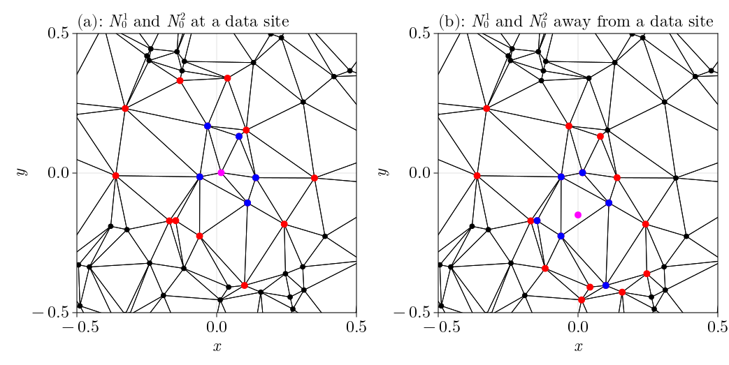
To choose the neighbourhood, define the $d$-times iterated neighbourhood of $\boldsymbol x_0$ by
\[N_0^d = \bigcup_{i \in N_0^{d-1}} N_i \setminus \{0\}, \quad N_0^1 = N_0.\]
Here, the neighbourhoods are the Delaunay neighbourhoods, not the natural neighbours – for points $\boldsymbol x_0$ that are not one of the existing data sites, natural neighbours are used instead. An example of $N_0^1$ and $N_0^2$ both at a data site and away from a data site is shown below, where $\boldsymbol x_0$ is shown in magenta, $N_0^1$ in blue, and $N_0^2$ in red (and also includes the blue points).
Gradients
Let's now use the notation defined above to define how gradients are generated in generate_derivatives, without having to estimate Hessians at the same time. The neighbourhood we use is $N_0^1$, and we take $\tilde f = z_0 + \tilde f_1$. We define the following weighted least squares problem for the estimates $\beta_x$, $\beta_y$ of $\partial f(\boldsymbol x_0)/\partial x$ and $\partial f(\boldsymbol x_0)/\partial y$, respectively:
\[(\beta_x, \beta_y) = \text{argmin}_{(\beta_x, \beta_y)} \sum_{i \in \mathcal N_0^1} W_i \left(\tilde z_i - \beta_1\tilde x_i - \beta_2\tilde y_i\right)^2,\]
where $W_i = 1/\|\boldsymbol x_i - \boldsymbol x_i\|^2$, $\tilde z_i = z_i-z_0$, $\tilde x_i=x_i-x_0$, and $\tilde y_i = y_i-y_0$. This weighted least squares problem is solved by solving the associated linear system $\tilde{\boldsymbol X}\boldsymbol{\beta} = \tilde{\boldsymbol z}$, where $\tilde{\boldsymbol X} \in \mathbb R^{m \times 2}$ is defined by $(\tilde{\boldsymbol X})_{i1} = \sqrt{W_i}(x_i - x_0)$ and $(\tilde{\boldsymbol X})_{i2} = \sqrt{W_i}(y_i - y_0)$, $\boldsymbol{\beta} = (\beta_1,\beta_2)^T$, and $\tilde{\boldsymbol z} = (\tilde z_1,\ldots,\tilde z_m)^T$.
Joint Gradients and Hessians
Hessians can similarly be estimated, although currently they must be estimated jointly with gradients. We take $\tilde f = z_0 + \tilde f_1 + \tilde f_2$ in the following discussion, although taking up to $\tilde f_3$ has an obvious extension. (The reason to also allow for estimating up to the cubic terms is because sometimes it provides better estimates for the Hessians than only going up to the quadratic terms – see the examples in Chapter 6 here.)
Defining $\beta_1 = \partial f(\boldsymbol x_0)/\partial x$, $\beta_2 = \partial f(\boldsymbol x_0)/\partial y$, $\beta_3 = \partial^2 f(\boldsymbol x_0)/\partial x^2$, $\beta_4 = \partial^2 f(\boldsymbol x_0)/\partial y^2$, and $\beta_5 = \partial^2 f(\boldsymbol x_0)/\partial x\partial y$, we have the following weighted least squares problem with $\boldsymbol{\beta}=(\beta_1,\beta_2,\beta_3,\beta_4,\beta_5)^T$:
\[\boldsymbol{\beta} = \text{argmin}_{\boldsymbol{\beta}} \sum_{i \in N_0^2} W_i\left(\tilde z_i - \beta_1\tilde x_i - \beta_2\tilde y_i - \frac12\beta_3\tilde x_i^2 - \frac12\beta_4\tilde y_i^2 - \beta_5\tilde x_i\tilde y_i\right)^2,\]
using similar notation as in the gradient case. (In the cubic case, use $N_0^3$ and go up to $\beta_9$, discarding $\beta_6,\ldots,\beta_9$ at the end.) The associated linear system in this case has matrix $\tilde{\boldsymbol X} \in \mathbb R^{m \times 2}$ ($m = |N_0^2|$) defined by $(\tilde{\boldsymbol X})_{i1} = \sqrt{W_i}\tilde x_i$, $(\tilde{\boldsymbol X})_{i2} = \sqrt{W_i}\tilde y_i$, $(\tilde{\boldsymbol X})_{i3} = \sqrt{W_i}\tilde x_i^2$, $(\tilde{\boldsymbol X})_{i4} = \sqrt{W_i}\tilde y_i^2$, and $(\tilde{\boldsymbol X})_{i5} = \sqrt{W_i}\tilde x_i\tilde y_i$.
Iterative Generation
Now we discuss iterative generation. Here, we suppose that we have already estimated gradients at all of the data sites $\boldsymbol x_i$ neighbouring $\boldsymbol x_0$ using the direct approach. To help with the notation, we will let $\boldsymbol g_i^1$ denote our initial estimate of the gradient at a point $\boldsymbol x_i$, and the gradient and Hessian that we are now estimating at $\boldsymbol x_0$ are given by $\boldsymbol g_0^2$ and $\boldsymbol H_0^2$, respectively.
We define the following loss function, where $\beta_i = 1/\|\boldsymbol x_i-\boldsymbol x_0\|$ and $\alpha \in (0, 1)$:
\[\begin{align*} \mathcal L(\boldsymbol g_0^2, \boldsymbol H_0^2) &= \sum_{i \in \mathcal N_0} W_i\left[\alpha \mathcal L_1^i(\boldsymbol g_0^2, \boldsymbol H_0^2)^2 + (1-\alpha)L_2^i(\boldsymbol g_0^2, \boldsymbol H_0^2)^2\right], \\ \mathcal L_1^i(\boldsymbol g_0^2, \boldsymbol H_0^2)^2 &= \left[\frac12(\boldsymbol x_i-\boldsymbol x_0)^T\boldsymbol H_0^2(\boldsymbol x_i - \boldsymbol x_0) + (\boldsymbol x_i-\boldsymbol x_0)^T\boldsymbol g_0^2 + z_0-z_i\right]^2, \\ \mathcal L_2^i(\boldsymbol g_0^2, \boldsymbol H_0^2) &= \left\|\boldsymbol H_0^2 \boldsymbol x_i + \boldsymbol g_0^2 - \boldsymbol g_i^1\right\|^2. \end{align*}\]
This objective function combines the losses between $\tilde f(\boldsymbol x_i)$ and $z_i$, and between $\boldsymbol \nabla \tilde f(\boldsymbol x_i)$ and $\boldsymbol g_i^1$, weighting them by some parameter $\alpha \in (0, 1)$ (typically $\alpha \approx 0.1$ is a reasonable default). After some basic algebra and calculus, it is possible to show that minimising $\mathcal L$ is the same as solving
\[\overline{\boldsymbol A}^T\overline{\boldsymbol w} + \overline{\boldsymbol B}^T\overline{\boldsymbol g}_1 + \overline{\boldsymbol C}^T\overline{\boldsymbol g}_2 = \left(\overline{\boldsymbol A}^T\overline{\boldsymbol A} + \overline{\boldsymbol B}^T\overline{\boldsymbol B} + \overline{\boldsymbol C}^T\overline{\boldsymbol C}\right)\boldsymbol \theta,\]
where we define:
\[\begin{align*} \tilde z_i &= z_i - z_0, \\ W_i &= \frac{1}{\|\boldsymbol x_i-\boldsymbol x_0\|^2},\\ \gamma_i &= \sqrt{\frac{\alpha}{W_i}}, \\ \gamma_i^\prime &= \sqrt{\frac{1-\alpha}{W_i}},\\ \overline{\boldsymbol A}_{i,:} &= \gamma_i \begin{bmatrix} x_i-x_0 & y_i-y_0 & \frac12(x_i-x_0)^2 & \frac12(y_i-y_0)^2 & (x_i-x_0)(y_i-y_0) \end{bmatrix}, \\ \overline{\boldsymbol B}_{i, :} &= \gamma_i^\prime \begin{bmatrix} 1 & 0 & x_i - x_0 & 0 & y_i - y_0 \end{bmatrix}, \\ \overline{\boldsymbol C}_{i, :} &= \gamma_i^\prime \begin{bmatrix} 0 & 1 & 0 & y_i-y_0 & x_i-x_0 \end{bmatrix}, \\ \overline{\boldsymbol w} &= \gamma_i \tilde z_i, \\ \overline{\boldsymbol g}_1 &= \gamma_i^\prime g_{i1}, \\ \overline{\boldsymbol g}_2 &= \gamma_i^\prime g_{i2}, \\ \boldsymbol{\bm\theta} &= \begin{bmatrix} \frac{\partial f(\boldsymbol x_0)}{\partial x} & \frac{\partial f(\boldsymbol x_0)}{\partial y} & \frac{\partial^2 f(\boldsymbol x_0)}{\partial x^2} & \frac{\partial f(\boldsymbol x_0)}{\partial y^2} & \frac{\partial f(\boldsymbol x_0)}{\partial x\partial y} \end{bmatrix}^T. \end{align*}\]
To solve this linear system, let
\[\boldsymbol D = \begin{bmatrix} \overline{\boldsymbol A} \\ \overline{\boldsymbol B} \\ \overline{\boldsymbol C} \end{bmatrix}, \quad \boldsymbol c = \begin{bmatrix} \overline{\boldsymbol w} \\ \overline{\boldsymbol g}_1 \\ \overline{\boldsymbol g}_2 \end{bmatrix},\]
so that $\boldsymbol D^T\boldsymbol D\boldsymbol\theta = \boldsymbol D^T\boldsymbol c$. These are just the normal equations for $\boldsymbol D\boldsymbol \theta = \boldsymbol c$, thus we can estimate the gradients and Hessians by simply solving $\boldsymbol D\boldsymbol \theta = \boldsymbol c$.
Generation Away from the Data Sites
It is possible to extend these ideas so that we can approximate the derivative at any point $\boldsymbol x_0 \in \mathcal C(\boldsymbol X)$. Using the associated interpolant, simply approximate $z_0$ with the value of the interpolant at $\boldsymbol x_0$, and then replace $W_i$ by $\lambda_i/\|\boldsymbol x_i-\boldsymbol x_0\|$, where $\lambda_i$ is the Sibson coordinate at $\boldsymbol x_i$ relative to $\boldsymbol x_0$. If using a direct approach to approximate gradients and Hessians, Sibson coordinates cannot be used (because you can't extend the weights out to $N_0^2$) and so $W_i$ remains as is in that case. Note that the $N_0$ neighbourhoods are now the sets of natural neighbours.