Interpolation
In this section, we give some of the mathematical background behind natural neighbour interpolation, and other interpolation methods provided from this package. The discussion here will be limited, but you can see this thesis or this Wikipedia article for more information. The discussion that follows is primarily sourced from the linked thesis. These ideas are implemented by the interpolate function.
Voronoi Tessellation
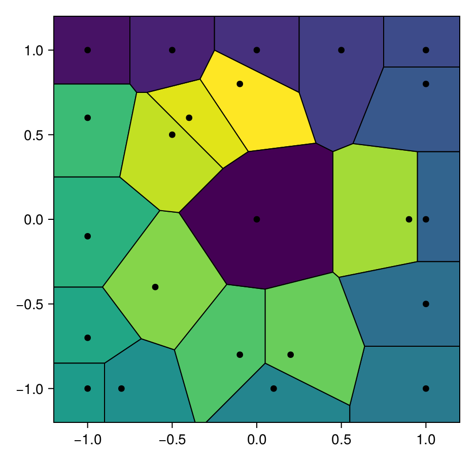
We need to first define the Voronoi tessellation. We consider some set of points $\boldsymbol X = \{\boldsymbol x_1, \ldots, \boldsymbol x_m\} \subseteq \mathbb R^2$. The Voronoi tessellation of $\boldsymbol X$, denoted $\mathcal V(\boldsymbol X)$, is a set of convex polygons $\{V_{\boldsymbol x_1}, \ldots, V_{\boldsymbol x_m}\}$, also called tiles, such that
\[\begin{equation*} V_{\boldsymbol x_i} = \{\boldsymbol x \in \mathbb R^2 : \|\boldsymbol x - \boldsymbol x_i\| \leq \|\boldsymbol x - \boldsymbol x_j\|,~ \boldsymbol x_j \in \boldsymbol X\}. \end{equation*}\]
In particular, any point in $V_{\boldsymbol x_i}$ is closer to $\boldsymbol x_i$ than it is to any other point in $\boldsymbol X$. We will also denote $V_{\boldsymbol x_i}$ by $V_i$. DelaunayTriangulation.jl is used to build $\mathcal V(\boldsymbol X)$. An example of a Voronoi tessellation is shown below.
Natural Neighbours
See that the tiles of the tessellation in the figure above intersect along a line, called the Voronoi facet, that we denote by $\mathcal F_{ij} = \mathcal V_i \cap \mathcal V_j$. Whenever $\mathcal F_{ij} \neq \emptyset$, we say that $\boldsymbol x_i$ and $\boldsymbol x_j$ are natural neighbours in $\boldsymbol X$. We denote the set of natural neighbours to a point $\boldsymbol x \in \boldsymbol X$ by $N(\boldsymbol x) \subseteq \boldsymbol X$, and we denote the corresponding indices by $N_i = \{j : \boldsymbol x_j \in N(\boldsymbol x_i)\}$.
Natural Neighbour Coordinates
We represent points locally using what are known as natural neighbour coordinates, which are based on the nearby Voronoi tiles. In particular, we make the following definition: Any set of convex coordinates $\boldsymbol \lambda$ (convex means that $\lambda_i \geq 0$ for each $i$) of $\boldsymbol x$ with respect to the natural neighbours $N(\boldsymbol x)$ of $\boldsymbol x$ that satisfies:
- $\lambda_i > 0 \iff \boldsymbol x_i \in N(\boldsymbol x)$,
- $\boldsymbol \lambda$ is continuous with respect to $\boldsymbol x$,
is called a set of natural neighbour coordinates of $\boldsymbol x$ in $\boldsymbol X$, or just the natural neighbour coordinates of $\boldsymbol x$, or the local coordinates of $\boldsymbol x$.
Natural Neighbour Interpolation
Now that we have some definitions, we can actually define the steps involved in natural neighbour interpolation. We are supposing that we have some data $(\boldsymbol x_i, z_i)$ for $i=1,\ldots,m$, and we want to interpolate this data at some point $\boldsymbol x_0 \in \mathcal C(\boldsymbol X)$, where $\boldsymbol X$ is the point set $(\boldsymbol x_1,\ldots,\boldsymbol x_m)$ and $\mathcal C(\boldsymbol X)$ is the convex hull of $\boldsymbol x$. We let $Z$ denote the function values $(z_1,\ldots,z_m)$.
The steps are relatively straight forward.
- First, compute local coordinates $\boldsymbol \lambda(\boldsymbol x_0)$ with respect to the natural neighbours $N(\boldsymbol x_0)$.
- Combine the values $z_i$ associated with $\boldsymbol x_i \in N(\boldsymbol x)$ using some blending function $\varphi(\boldsymbol \lambda, Z)$.
To consider the second step, note that a major motivation for working with local coordinates is the following fact: The coordinates $\boldsymbol \lambda$ that we compute can be used to represent our point $\boldsymbol x_0$ as $\boldsymbol x_0 = \sum_{i \in N_0} \lambda_i(\boldsymbol x_0)\boldsymbol x_i$, a property known as the local coordinates property (Sibson, 1980), or the natural neighbour coordinates property if $\boldsymbol \lambda$ is convex (as we assume them to be).
In particular, the coordinates $\boldsymbol \lambda$ determine how much each point $\boldsymbol x_i \in N(\boldsymbol x_0)$ contributes to the representation of our query point $\boldsymbol x_0$, hence the term "natural". So, a natural interpolant is to simply take this linear combination and replace $\boldsymbol x_i$ by $z_i$, giving the scattered data interpolant
\[f(\boldsymbol x_0) = \sum_{i \in N_0} \lambda_i z_i.\]
Note that the natural neighbour coordinates property only works for points in the convex hull of $\boldsymbol X$ (otherwise $\boldsymbol \lambda$ is not convex), hence the restriction $\boldsymbol x_0 \in \mathcal C(\boldsymbol X)$.
Some Local Coordinates
Let us now define all the coordinates we provide in this package.
Nearest Neighbours
To represent a point $\boldsymbol x_0$, we can use what are known as nearest neighbour coordinates, which simply assigns a weight of $1$ to the generator of the tile that $\boldsymbol x_0$ is in:
\[\lambda_i^{\text{NEAR}} = \begin{cases} 1 & \boldsymbol x_0 \in \mathcal V_i, \\ 0 & \text{otherwise}. \end{cases}\]
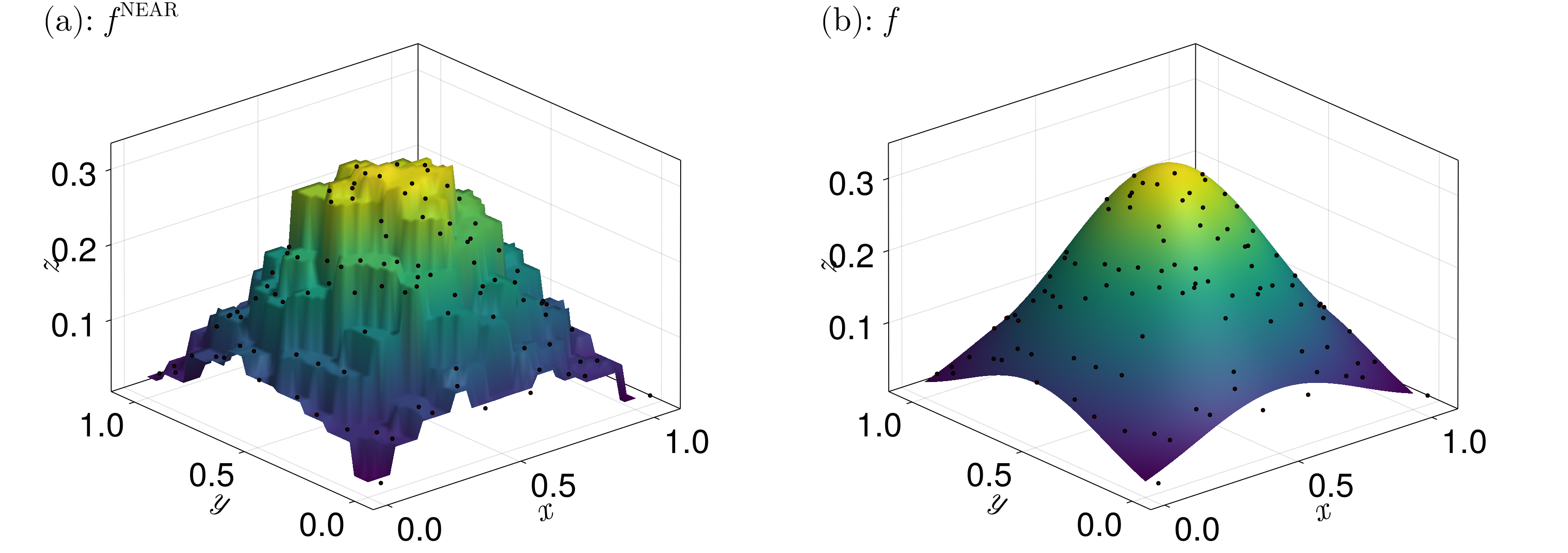
The resulting scattered data interpolant $f^{\text{NEAR}}$ is then just
\[f^{\text{NEAR}}(\boldsymbol x) = z_i, \]
where $\boldsymbol x \in \mathcal V_i$. An example of what this interpolant looks like is given below.
Laplace Coordinates
Here we introduce Laplace coordinates, also known as non-Sibsonian coordinates. To define these coordinates, let us take some tessellation $\mathcal V(\boldsymbol X)$ and see what happens when we add a point into it.
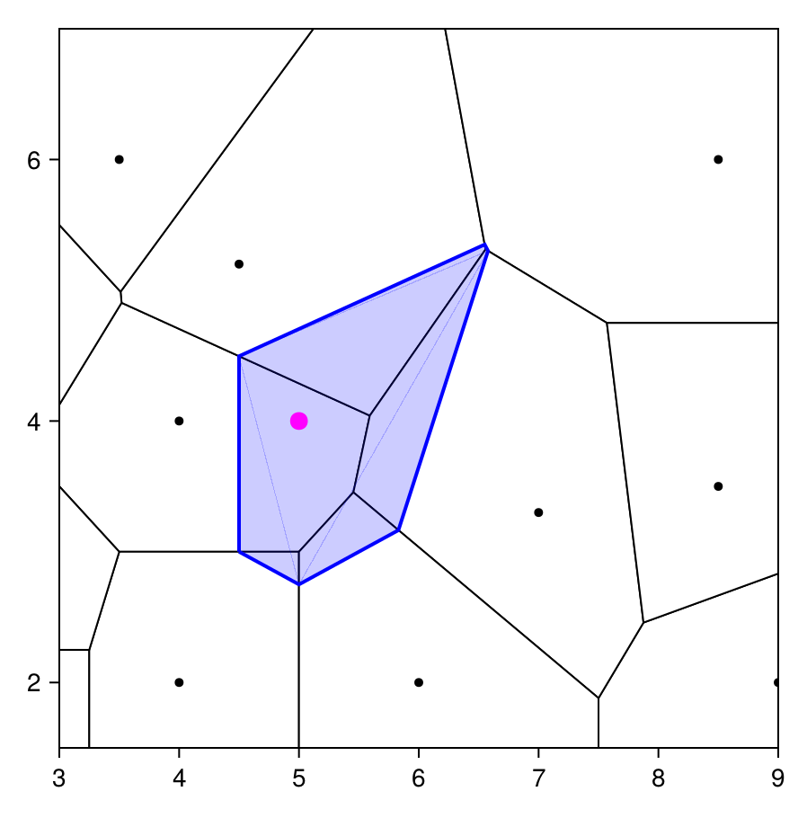
In the figure above, the tiles with the black boundaries and no fill are the tiles of the original tessellation, and we show the tile that would be created by some query point $\boldsymbol x_0$ (the magenta point) with a blue tile. We see that the insertion of $\boldsymbol x_0$ into the tessellation has intersected some of the other tiles, in particular it has modified only the tiles corresponding to its natural neighbours in $N(\boldsymbol x_0)$.
For a given generator $\boldsymbol x_i \in N(\boldsymbol x_0)$, we see that there is a corresponding blue line passing through its tile. Denote this blue line by $\mathcal F_{0i}$, and let $r_i = \|\boldsymbol x_0 - \boldsymbol x_i\|$. With this definition, we define
\[\lambda_i^{\text{LAP}} = \frac{\hat\lambda_i^{\text{LAP}}}{\sum_{j \in N_0} \hat\lambda_j^{\text{LAP}}}, \quad \hat\lambda_i^{\text{LAP}} = \frac{\ell(\mathcal F_{0i})}{r_i},\]
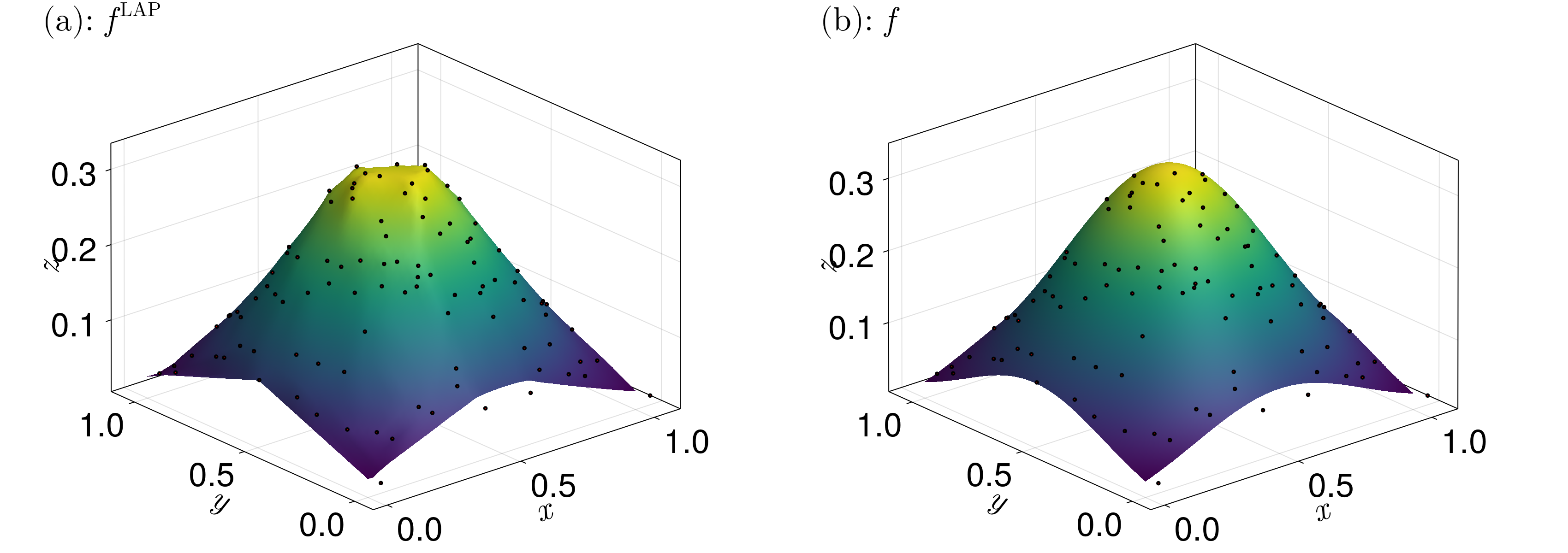
where $\ell(\mathcal F_{0i})$ is the length of the facet $\mathcal F_{0i}$. In particular, $\hat\lambda_i^{\text{LAP}}$ is the ratio of the blue line inside the tile and the distance between the generator $\boldsymbol x_i$ and the query point $\boldsymbol x_0$. These coordinates are continuous in $\mathcal C(\boldsymbol X)$ with derivative discontinuities at the data sites $\boldsymbol X$. The resulting interpolant $f^{\text{LAP}}$ inherits these properties, where
\[f^{\text{LAP}}(\boldsymbol x_0) = \sum_{i \in N_0} \lambda_i^{\text{LAP}}z_i.\]
This interpolant has linear precision, meaning it reproduces linear functions.
An example of what this interpolant looks like is given below.
Sibson Coordinates
Now we consider Sibson's coordinates. These coordinates are similar to Laplace's coordinates, except we consider the areas rather than lengths for the facets. In particular, let us return to the figure above, reprinted below for convenience:
The idea is to consider how much area this new blue tile "steals" from the tiles of its natural neighbours. Based on the following identity (Sibson, 1980),
\[\text{Area}(\mathcal V_{\boldsymbol x_0}) \boldsymbol x = \sum_{i \in N_0} \text{Area}(\mathcal V_{\boldsymbol x} \cap \mathcal V_{\boldsymbol x_i}^{\boldsymbol x_0})\boldsymbol x_i,\]
where $\mathcal V_{\boldsymbol x_0}$ is the new tile shown in blue, and $\mathcal V_{\boldsymbol x_i}^{\boldsymbol x_0}$ is the tile associated with $\boldsymbol x_i$ in the original tessellation, i.e. prior to the insertion of $\boldsymbol x_0$, we define Sibson's coordinates as
\[\lambda_i^{\text{SIB}} = \frac{\hat\lambda_i^{\text{SIB}}}{\sum_{j \in N_0} \hat\lambda_j^{\text{SIB}}}, \quad \hat\lambda_i^{\text{SIB}} = \text{Area}(\mathcal V_{\boldsymbol x_0} \cap \mathcal V_{\boldsymbol x_i}^{\boldsymbol x_0}).\]
A clearer way to write this is as
\[\lambda_i^{\text{SIB}} = \frac{A(\boldsymbol x_i)}{A(\boldsymbol x)},\]
where $A(\boldsymbol x_i)$ is the area of the intersection between the original tile for $\boldsymbol x_i$ and the new tile at $\boldsymbol x_0$, and $A(\boldsymbol x)$ is the total area of the new blue tile. These coordinates are $C^1$ continuous in $\mathcal C(\boldsymbol X) \setminus \boldsymbol X$, with derivative discontinuities at the data sites, and so too is the interpolant
\[f^{\text{SIB}}(\boldsymbol x_0) = \sum_{i \in N_0} \lambda_i^{\text{SIB}}z_i.\]
We may also use $f^{\text{SIB}0}$ and $\lambda_i^{\text{SIB}0}$ rather than $f^{\text{SIB}}$ and $\lambda_i^{\text{SIB}}$, respectively.
This interpolant has linear precision, meaning it reproduces linear functions.
An example of what this interpolant looks like is given below.
Our implementation of these coordinates follows this article with some simple modifications.
Triangle Coordinates
Now we define triangle coordinates. These are not actually natural coordinates (they are not continuous in $\boldsymbol x$), but they just give a nice comparison with other methods. The idea is to interpolate based on the barycentric coordinates of the triangle that the query point is in, giving rise to a piecewise linear interpolant over $\mathcal C(\boldsymbol X)$.
Let us take our query point $\boldsymbol x=(x,y)$ and suppose it is in some triangle $V$ with coordinates $\boldsymbol x_1 = (x_1,y_1)$, $\boldsymbol x_2 = (x_2,y_2)$, and $\boldsymbol x_3=(x_3,y_3)$. We can then define:
\[\begin{align*} \Delta &= (y_2-y_3)(x_1-x_3)+(x_3-x_2)(y_1-y_3), \\ \lambda_1 &= \frac{(y_2-y_3)(x-x_3)+(x_3-x_2)(y-y_3)}{\Delta}, \\ \lambda_2 &= \frac{(y_3-y_1)(x-x_3) + (x_1-x_3)(y-y_3)}{\Delta}, \\ \lambda_3 &= 1-\lambda_1-\lambda_2. \end{align*}\]
With these definitions, our interpolant is
\[f^{\text{TRI}}(\boldsymbol x) = \lambda_1z_1 + \lambda_2z_2 + \lambda_3z_3.\]
(Of course, the subscripts would have to be modified to match the actual indices of the points rather than assuming them to be $\boldsymbol x_1$, $\boldsymbol x_2$, and $\boldsymbol x_3$.) This is the same interpolant used in FiniteVolumeMethod.jl.
An example of what this interpolant looks like is given below.
Smooth Interpolation
All the derived interpolants above are not differentiable at the data sites. Here we describe some interpolants that are differentiable at the data sites.
Sibson's $C^1$ Interpolant
Sibson's $C^1$ interpolant, which we call Sibson-1 interpolation, extends on Sibson coordinates above, also called Sibson-0 coordinates, is $C^1$ at the data sites. A limitation of it is that it requires an estimate of the gradient $\boldsymbol \nabla_i$ at the data sites $\boldsymbol x_i$, which may be estimated using the derivative generation techniques described in the sidebar.
Following Bobach's thesis or Flötotto's thesis, the Sibson-1 interpolant $f^{\text{SIB}1}$ is a linear combination of $f^{\text{SIB}0} \equiv f^{\text{SIB}}$ and another interpolant $\xi$. We define:
\[\begin{align*} r_i &= \|\boldsymbol x_0-\boldsymbol x_i\|, \\ \gamma_i &= \frac{\lambda_i^{\text{SIB}0}}{r_i}, \\ \zeta_i &= z_i + (\boldsymbol x_0 - \boldsymbol x_i)^T\boldsymbol\nabla_i, \\ \zeta &= \frac{\sum_{i\in N_0} \gamma_i\zeta_i}{\sum_{i\in N_0} \gamma_i}, \\ \alpha &= \frac{\sum_{i \in N_0} \lambda_i^{\text{SIB}0}r_i}{\sum_{i \in N_0} \gamma_i}, \\ \beta &= \sum_{i \in N_0} \lambda_i^{\text{SIB}0}r_i^2. \end{align*}\]
Our interpolant is then defined by
\[f^{\text{SIB}1}(\boldsymbol x_0) = \frac{\alpha f^{\text{SIB}0} + \beta\zeta}{\alpha + \beta}.\]
This interpolant exactly reproduces spherical quadratics $\boldsymbol x \mapsto \mu(\boldsymbol x - \boldsymbol a)^T(\boldsymbol x - \boldsymbol a)$.
An example of what this interpolant looks like is given below.
Notice that the peak of the function is much smoother than it was in the other interpolant examples.
Farin's $C^1$ Interpolant
Farin's $C^1$ interpolant, introduced by Farin (1990), is another interpolant with $C^1$ continuity at the data sites provided we have estimates of the gradients $\boldsymbol \nabla_i$ at the data sites (see the sidebar for derivative generation methods), and also makes use of the Sibson-0 coordinates. Typically these coordinates are described in the language of Bernstein-Bézier simplices (as in Bobach's thesis or Flötotto's thesis and Farin's original paper), this language makes things more complicated than they need to be. Instead, we describe the interpolant using symmetric homogeneous polynomials, as in Hiyoshi and Sugihara (2004, 2007). See the references mentioned above for a derivation of the interpolant we describe below.
Let $\boldsymbol x_0$ be some point in $\mathcal C(\boldsymbol X)$ and let $N_0$ be the natural neighbourhood around $\boldsymbol x_0$. We let the natural coordinates be given by Sibson's coordinates $\boldsymbol \lambda = (\lambda_1,\ldots,\lambda_n)$ with corresponding natural neighbours $\boldsymbol x_1,\ldots,\boldsymbol x_n$ (rearranging the indices accordingly to avoid using e.g. $i_1,\ldots, i_n$), where $n = |N_0|$. We define a homogeneous symmetric polynomial
\[f(\boldsymbol x_0) = \sum_{i \in N_0}\sum_{j \in N_0}\sum_{k \in N_0} f_{ijk}\lambda_i\lambda_j\lambda_k,\]
where the coefficients $f_{ijk}$ are symmetric so that they can be uniquely determined. We define $z_{i, j} = \boldsymbol \nabla_i^T \overrightarrow{\boldsymbol x_i\boldsymbol x_j}$, where $\boldsymbol \nabla_i$ is the estimate of the gradient at $\boldsymbol x_i \in N(\boldsymbol x_0) \subset \boldsymbol X$ and $\overrightarrow{\boldsymbol x_i\boldsymbol x_j} = \boldsymbol x_j - \boldsymbol x_i$. Then, define the coefficients (using symmetry to permute the indices to the standard forms below):
\[\begin{align*} f_{iii} &= z_i, \\ f_{iij} &= z_i + \frac{1}{3}z_{i,j}, \\ f_{ijk} &= \frac{z_i+z_j+z_k}{3} + \frac{z_{i,j}+z_{i,k}+z_{j,i}+z_{j,k}+z_{k,i}+z_{k,j}}{12}, \end{align*}\]
where all the $i$, $j$, and $k$ are different. The resulting interpolant $f$ is Farin's $C^1$ interpolant, $f^{\text{FAR}} = f$, and has quadratic precision so that it reproduces quadratic polynomials.
Let us describe how we actually evaluate $\sum_{i \in N_0}\sum_{j \in N_0}\sum_{k \in N_0} f_{ijk}\lambda_i\lambda_j\lambda_k$ efficiently. Write this as
\[f^{\text{FAR}}(\boldsymbol x_0) = \sum_{1 \leq i, j, k \leq n} f_{ijk}\lambda_i\lambda_j\lambda_k.\]
This looks close to the definition of a complete homogeneous symmetric polynomial. This page shows the identity
\[\sum_{1 \leq i \leq j \leq k \leq n} X_iX_kX_j = \sum_{1 \leq i, j, k \leq n} \frac{m_i!m_j!m_k!}{3!}X_iX_jX_k,\]
where $m_\ell$ is the multiplicity of $X_\ell$ in the summand, e.g. if the summand is $X_i^2X_k$ then $m_i=2$ and $m_k = 1$. Thus, transforming the variables accordingly, we can show that
\[f^{\text{FAR}}(\boldsymbol x_0) = 6\underbrace{\sum_{i=1}^n\sum_{j=i}^n\sum_{k=j}^n}_{\sum_{1 \leq i \leq j \leq k \leq n}} \tilde f_{ijk}\lambda_i\lambda_j\lambda_k,\]
where $\tilde f_{iii} = f_{iii}/3! = f_{iii}/6$, $\tilde f_{iij} = f_{iij}/2$, and $\tilde f_{ijk} = f_{ijk}$. This is the implementation we use.
Hiyoshi's $C^2$ Interpolant
Hiyoshi's $C^2$ interpolant is similar to Farin's $C^1$ interpolant, except now we have $C^2$ continuity at the data sites and we now, in addition to requiring estimates of the gradients $\boldsymbol \nabla_i$ at the data sites, require estimates of the Hessians $\boldsymbol H_i$ at the data sites (see the sidebar for derivative generation methods). As with Farin's $C^1$ interpolant, we use the language of homogeneous symmetric polynomials rather than Bernstein-Bézier simplices in what follows. There are two definitions of Hiyoshi's $C^2$ interpolant, the first being given by Hiyoshi and Sugihara (2004) and described by Bobach, and the second given three years later again by Hiyoshi and Sugihara (2007). We use the 2007 definition - testing shows that they are basically the same, anyway.
Like in the previous section, w let $\boldsymbol x_0$ be some point in $\mathcal C(\boldsymbol X)$ and let $N_0$ be the natural neighbourhood around $\boldsymbol x_0$. We let the natural coordinates be given by Sibson's coordinates $\boldsymbol \lambda = (\lambda_1,\ldots,\lambda_n)$ with corresponding natural neighbours $\boldsymbol x_1,\ldots,\boldsymbol x_n$ (rearranging the indices accordingly to avoid using e.g. $i_1,\ldots, i_n$), where $n = |N_0|$. We define
\[z_{i, j} = \boldsymbol \nabla_i^T\overrightarrow{\boldsymbol x_i\boldsymbol x_j}, \qquad z_{i, jk} = \overrightarrow{\boldsymbol x_i\boldsymbol x_j}^T\boldsymbol H_i\overrightarrow{\boldsymbol x_i\boldsymbol x_k}.\]
Hiyoshi's $C^2$ interpolant, written $f^{\text{HIY}}$ (or later $f^{\text{HIY}2}$, if ever we can get Hiyoshi's $C^k$ interpolant on $\mathcal C(\boldsymbol X) \setminus \boldsymbol X$ implemented –- see Hiyoshi and Sugihara (2000, 2002), Bobach, Bertram, Umlauf (2006), and Chapter 3.2.5.5 and Chapter 5.5. of Bobach's thesis), is defined by the homogeneous symmetric polynomial
\[f^{\text{HIY}}(\boldsymbol x_0) = \sum_{1 \leq i,j,k,\ell,m \leq n} f_{ijk\ell m}\lambda_i\lambda_j\lambda_k\lambda_\ell\lambda_m,\]
where we define the coefficients (using symmetry to permute the indices to the standard forms below):
\[\begin{align*} f_{iiiii} &= z_i, \\ f_{iiiij} &= z_i + \frac15z_{i,j}, \\ f_{iiijj} &= z_i + \frac25z_{i,j} + \frac{1}{20}z_{i,jj}, \\ f_{iiijk} &= z_i + \frac15\left(z_{i, j} + z_{i, k}\right) + \frac{1}{20}z_{i, jk}, \\ f_{iijjk} &= \frac{13}{30}\left(z_i + z_j\right) + \frac{2}{15}z_k + \frac{1}{9}\left(z_{i, j} + z_{j, i}\right) + \frac{7}{90}\left(z_{i, k} + z_{j, k}\right) \\&+ \frac{2}{45}\left(z_{k, i} + z_{k, j}\right) + \frac{1}{45}\left(z_{i, jk} + z_{j, ik} + z_{k, ij}\right), \\ f_{iijk\ell} &= \frac12z_i + \frac16\left(z_j + z_k + z_\ell\right) + \frac{7}{90}\left(z_{i, j} + z_{i, k} + z_{i, \ell}\right) \\&+ \frac{2}{45}\left(z_{j, i} + z_{k, i} + z_{\ell, i}\right) + \frac{1}{30}\left(z_{j, k} + z_{j, \ell} + z_{k, j} + z_{k, \ell} + z_{\ell, j} + z_{j, k}\right) \\ &+ \frac{1}{90}\left(z_{i, jk} + z_{i, j\ell} + z_{i, k\ell}\right) + \frac{1}{90}\left(z_{j, ik} + z_{j, i\ell} + z_{k, ij} + z_{k, i\ell} + z_{\ell, ij} + z_{\ell, ik}\right) \\&+ \frac{1}{180}\left(z_{j, k\ell} + z_{k, j\ell} + z_{\ell, jk}\right), \\ f_{ijk\ell m} &= \frac{1}{5}\left(z_i + z_j + z_k + z_\ell + z_m\right) \\ &+ \frac{1}{30}\left(z_{i, j} + z_{i, k} + z_{i, \ell} + z_{i, m} + z_{j, i} + \cdots + z_{m, \ell}\right) \\ &+ \frac{1}{180}\left(z_{i, jk} + z_{i, j\ell} + z_{i, jm} + z_{i, k\ell} + z_{i, km} + z_{i, \ell m} + z_{j, i\ell} + \cdots + z_{mk\ell}\right), \end{align*}\]
where all the $i$, $j$, $k$, $\ell$, and $m$ are different. To evaluate $f^{\text{HIY}}$, we use the same relationship between $f^{\text{HIY}}$ and complete homogeneous symmetric polynomials to write
\[f^{\text{HIY}}(\boldsymbol x_0) = 120\sum_{1 \leq i \leq j \leq k \leq \ell \leq m \leq n} \tilde f_{ijk \ell m} \lambda_i\lambda_j\lambda_k\lambda_\ell \lambda_m,\]
where $\tilde f_{iiiii} = f_{iiiii}/5! = f_{iiiii}/120$, $\tilde f_{iiiij} = f_{iiiij}/24$, $\tilde f_{iijjj} = f_{iijjj}/12$, $\tilde f_{iijjk} = f_{iijjk}/4$, $\tilde f_{iijk\ell} = f_{iijk\ell}/2$, and $\tilde f_{ijk\ell m} = f_{ijk\ell m}$.
This interpolant has cubic precision, meaning it can recover cubic polynomials. Note that this sum has
\[\sum_{i=1}^n\sum_{j=i}^n\sum_{k=j}^n\sum_{\ell=k}^n\sum_{m=k}^n 1 = \frac{n^5}{120} + \frac{n^4}{12} + \cdots = \mathcal O(n^5)\]
terms, which could cause issues with many natural neighbours. For example, with $n = 20$ we have $n^5 = 3,200,000$. In fact, as discussed in Section 6.5 of Bobach's thesis, more than 150 million operations could be required with $n = 20$. We discuss benchmark results in the comparison section of the sidebar.
Regions of Influence
The region of influence for the natural neighbour coordinates associated with a point $\boldsymbol x_i$ is the interior the union of all circumcircles coming from the triangles of the underlying triangulation that pass through $\boldsymbol x_i$. We can visualise this for the coordinates we define above below. (this region of influence definition not necessarily generalise to the triangle and nearest neighbour coordinates, but we still compare them).
We take a set of data sites in $[-1, 1]^2$ such that all function values are zero except for $z_1 = 0$ with $\boldsymbol x_1 = \boldsymbol 0$. Using this setup, we obtain the following results (see also Figure 3.6 of Bobach's thesis linked previously):
We can indeed see the effect of the region of influence about this single point $\boldsymbol x_1$. Note also that $f^{\text{SIB}1}$ is much smoother than the others.
Extrapolation
An important consideration is extrapolation. Currently, all the methods above assume that the query point $\boldsymbol x_0$ is in $\mathcal C(\boldsymbol X)$, and the interpolation near the boundary of $\mathcal C(\boldsymbol X)$ often has some weird effects. There are many approaches available for extrapolation, such as with ghost points, although these are not implemented in this package (yet!).
The approach we take for any point outside of $\mathcal C(\boldsymbol X)$, or on $\partial\mathcal C(\boldsymbol X)$, is to find the ghost triangle that $\boldsymbol x_0$ is in (ghost triangles are defined here in the DelaunayTriangulation.jl documentation), which will have some boundary edge $\boldsymbol e_{ij}$. (Similarly, if $\boldsymbol x_0 \in \partial \mathcal C(\boldsymbol X)$, $\boldsymbol e_{ij}$ is the boundary edge that it is on.) We then simply use two-point interpolation, letting
\[f(\boldsymbol x_0) \approx \lambda_iz_i + \lambda_jz_j,\]
where $\lambda_i = 1-t$, $\lambda_j = t$, $\ell = \|x_i - \boldsymbol x_j\|$, and $t = [(x_0 - x_i)(x_j - x_i) + (y_0 - y_i)(y_j - y_i)]/\ell^2$. Note also that in this definition of $t$ we have projected $\boldsymbol x_0$ onto the line through $\boldsymbol x_i$ and $\boldsymbol x_j$ – this projection is not necessarily on $\boldsymbol e_{ij}$, though, so $t$ will not always be in $[0, 1]$, meaning the coordinates are not guaranteed to be (and probably won't be) convex.
This extrapolation will not always be perfect, but it is good enough until we implement more sophisticated methods. If you want to disable this approach, just use the project = false keyword argument when evaluating your interpolant.
Similarly, if you have points defining a boundary of some domain that isn't necessarily convex, the function identify_exterior_points may be useful to you, provided you have represented your boundary as defined here in DelaunayTriangulation.jl. See the Switzerland example in the sidebar for more information.